📊 AdaBoost
XGBoost, LightGBM and CatBoost are all gradient boosting: each tree is fitted to the gradient of a loss. AdaBoost came first, and boosts a different way — by reweighting the data.
The idea, from 1995, is startlingly simple:
Train a weak model. Find which points it got wrong. Make those points matter more. Train another. Repeat. Give each model a vote proportional to how good it was.
$$F(x) = \operatorname{sign}\!\left(\sum_{m=1}^{M}\alpha_m h_m(x)\right)$$
A weak learner need only beat chance — here, a decision stump: a tree of depth 1, one question. The remarkable result is that a sequence of such stumps, correctly weighted, becomes a strong classifier.
Everything below is computed by hand for three rounds — every sample weight, every $\alpha$, every reweighting — then checked against scikit-learn.
Display helpers ready: banner, step, check, expand, show_matrix, show_matmul, show_elementwise.
1. The Data and the Weak Learner
The same 12 EEG recordings as the tree walkthroughs. AdaBoost uses labels in $\{-1, +1\}$, because that convention makes $y \cdot h(x)$ positive exactly when the prediction is right — which the $\alpha$ formula relies on.
12 recordings x 3 features

    id      region   line_length    spike_rate           age   y_class    y_reg
-------------------------------------------------------------------------------
 rec00     frontal          12.0           0.5          24.0         0      0.2
 rec01    temporal          15.0           1.2          31.0         0      0.5
 rec02    temporal          42.0           6.8          58.0         1      6.4
 rec03   occipital          38.0           5.1          47.0         1      4.8
 rec04     frontal          11.0           0.3          19.0         0      0.1
 rec05    temporal          55.0           8.2          63.0         1      9.1
 rec06   occipital          40.0           1.9          35.0         1      3.5
 rec07    temporal          47.0           7.4          52.0         1      7.2
 rec08     frontal          14.0           0.8          28.0         0      0.3
 rec09   occipital          51.0           6.1          60.0         1      6.9
 rec10     frontal          45.0           2.4          41.0         0      1.6
 rec11    temporal          35.0           4.7          30.0         1      4.1
-------------------------------------------------------------------------------

class balance: 5 negative, 7 positive
y_reg mean = 3.7250, std = 3.0518
labels recoded: [-1 -1  1  1 -1  1  1  1 -1  1 -1  1]

the best single stump on UNIFORM weights (w = 1/12 each):

   rule : predict -1 if line_length <= 25.00, else +1
   weighted error : 0.083333
   accuracy       : 0.9167

A single stump gets 11 of 12 right. It is 'weak' - better than the 50% a coin would
manage, and not much more. That is all AdaBoost requires.
2. The Three Formulas
Each round does exactly three things:
1. Weighted error of the new weak learner:
$$\varepsilon_m = \sum_{i} w_i \,\mathbb{1}[\,h_m(x_i) \ne y_i\,]$$
2. Its vote, derived by minimising exponential loss:
$$\alpha_m = \frac{1}{2}\ln\!\left(\frac{1-\varepsilon_m}{\varepsilon_m}\right)$$
3. Reweight, then renormalise so the weights sum to 1:
$$w_i \leftarrow w_i \exp\!\big(-\alpha_m y_i h_m(x_i)\big)$$
Read the $\alpha$ formula — it does something sensible at every value:
| $\varepsilon$ | $\alpha$ | meaning |
|---|---|---|
| 0.01 | $+2.30$ | nearly perfect → large vote |
| 0.40 | $+0.20$ | slightly useful → small vote |
| 0.50 | $0$ | a coin → no vote at all |
| 0.70 | $-0.42$ | worse than chance → negative vote — believe its opposite |
error eps       alpha     exp(+a)     exp(-a)                             reading
----------------------------------------------------------------------------------
       0.01      2.2976      9.9499      0.1005          nearly perfect -> big vote
       0.10      1.0986      3.0000      0.3333                useful -> solid vote
       0.25      0.5493      1.7321      0.5774                useful -> solid vote
       0.40      0.2027      1.2247      0.8165         barely useful -> small vote
       0.49      0.0200      1.0202      0.9802         barely useful -> small vote
       0.50      0.0000      1.0000      1.0000                   a coin -> ignored
       0.51     -0.0200      0.9802      1.0202       worse than chance -> inverted
       0.70     -0.4236      0.6547      1.5275       worse than chance -> inverted
----------------------------------------------------------------------------------

the reweighting factor exp(-alpha*y*h):
   correct  (y*h = +1) -> multiply weight by exp(-alpha)  <- shrinks
   wrong    (y*h = -1) -> multiply weight by exp(+alpha)  <- grows

   at eps = 0.25, alpha = 0.5493:
      correct points shrink by 0.5774x
      wrong   points grow  by 1.7321x
      ratio: a mistake becomes 3.00x more important than a hit


why that alpha? it minimises the exponential loss.
With Z(a) = sum_i w_i exp(-a*y_i*h_i) = (1-eps)e^-a + eps*e^a,
setting dZ/da = 0 gives a = 0.5*ln((1-eps)/eps). Checked numerically:

   eps = 0.1: grid minimum at a = +1.09860, formula gives +1.09861   MATCH: True
   eps = 0.25: grid minimum at a = +0.54930, formula gives +0.54931   MATCH: True
   eps = 0.4: grid minimum at a = +0.20270, formula gives +0.20273   MATCH: True
3. Three Rounds, Every Number
==============================================================================
  ROUND 1
==============================================================================

chosen stump: predict -1 if line_length <= 25.00

    id    weight w_i     y    h(x)     y*h   correct?    w if wrong
------------------------------------------------------------------
 rec00      0.083333    -1      -1       1        yes      0.000000
 rec01      0.083333    -1      -1       1        yes      0.000000
 rec02      0.083333     1       1       1        yes      0.000000
 rec03      0.083333     1       1       1        yes      0.000000
 rec04      0.083333    -1      -1       1        yes      0.000000
 rec05      0.083333     1       1       1        yes      0.000000
 rec06      0.083333     1       1       1        yes      0.000000
 rec07      0.083333     1       1       1        yes      0.000000
 rec08      0.083333    -1      -1       1        yes      0.000000
 rec09      0.083333     1       1       1        yes      0.000000
 rec10      0.083333    -1       1      -1         NO      0.083333
 rec11      0.083333     1       1       1        yes      0.000000
------------------------------------------------------------------
   sum      1.000000

   eps = sum of weights on WRONG points
       = 0.0833 = 0.083333

   alpha = 0.5 * ln((1 - 0.083333) / 0.083333)
         = 0.5 * ln(11.000000) = 1.198948

   reweight: w_i * exp(-alpha * y_i * h_i)
      correct -> x exp(-1.1989) = 0.301511
      wrong   -> x exp(+1.1989) = 3.316625
   normalising constant Z = 0.552771

    id        old w      factor    new (raw)    new (norm)     change
------------------------------------------------------------------
 rec00     0.083333    0.301511     0.025126      0.045455     0.545x
 rec01     0.083333    0.301511     0.025126      0.045455     0.545x
 rec02     0.083333    0.301511     0.025126      0.045455     0.545x
 rec03     0.083333    0.301511     0.025126      0.045455     0.545x
 rec04     0.083333    0.301511     0.025126      0.045455     0.545x
 rec05     0.083333    0.301511     0.025126      0.045455     0.545x
 rec06     0.083333    0.301511     0.025126      0.045455     0.545x
 rec07     0.083333    0.301511     0.025126      0.045455     0.545x
 rec08     0.083333    0.301511     0.025126      0.045455     0.545x
 rec09     0.083333    0.301511     0.025126      0.045455     0.545x
 rec10     0.083333    3.316625     0.276385      0.500000     6.000x
 rec11     0.083333    0.301511     0.025126      0.045455     0.545x
------------------------------------------------------------------
   weights sum to 1.0000000000

==============================================================================
  ROUND 2
==============================================================================

chosen stump: predict -1 if spike_rate <= 3.55

    id    weight w_i     y    h(x)     y*h   correct?    w if wrong
------------------------------------------------------------------
 rec00      0.045455    -1      -1       1        yes      0.000000
 rec01      0.045455    -1      -1       1        yes      0.000000
 rec02      0.045455     1       1       1        yes      0.000000
 rec03      0.045455     1       1       1        yes      0.000000
 rec04      0.045455    -1      -1       1        yes      0.000000
 rec05      0.045455     1       1       1        yes      0.000000
 rec06      0.045455     1      -1      -1         NO      0.045455
 rec07      0.045455     1       1       1        yes      0.000000
 rec08      0.045455    -1      -1       1        yes      0.000000
 rec09      0.045455     1       1       1        yes      0.000000
 rec10      0.500000    -1      -1       1        yes      0.000000
 rec11      0.045455     1       1       1        yes      0.000000
------------------------------------------------------------------
   sum      1.000000

   eps = sum of weights on WRONG points
       = 0.0455 = 0.045455

   alpha = 0.5 * ln((1 - 0.045455) / 0.045455)
         = 0.5 * ln(21.000000) = 1.522261

   reweight: w_i * exp(-alpha * y_i * h_i)
      correct -> x exp(-1.5223) = 0.218218
      wrong   -> x exp(+1.5223) = 4.582576
   normalising constant Z = 0.416598

    id        old w      factor    new (raw)    new (norm)     change
------------------------------------------------------------------
 rec00     0.045455    0.218218     0.009919      0.023810     0.524x
 rec01     0.045455    0.218218     0.009919      0.023810     0.524x
 rec02     0.045455    0.218218     0.009919      0.023810     0.524x
 rec03     0.045455    0.218218     0.009919      0.023810     0.524x
 rec04     0.045455    0.218218     0.009919      0.023810     0.524x
 rec05     0.045455    0.218218     0.009919      0.023810     0.524x
 rec06     0.045455    4.582576     0.208299      0.500000    11.000x
 rec07     0.045455    0.218218     0.009919      0.023810     0.524x
 rec08     0.045455    0.218218     0.009919      0.023810     0.524x
 rec09     0.045455    0.218218     0.009919      0.023810     0.524x
 rec10     0.500000    0.218218     0.109109      0.261905     0.524x
 rec11     0.045455    0.218218     0.009919      0.023810     0.524x
------------------------------------------------------------------
   weights sum to 1.0000000000

==============================================================================
  ROUND 3
==============================================================================

chosen stump: predict +1 if line_length <= 43.50

    id    weight w_i     y    h(x)     y*h   correct?    w if wrong
------------------------------------------------------------------
 rec00      0.023810    -1       1      -1         NO      0.023810
 rec01      0.023810    -1       1      -1         NO      0.023810
 rec02      0.023810     1       1       1        yes      0.000000
 rec03      0.023810     1       1       1        yes      0.000000
 rec04      0.023810    -1       1      -1         NO      0.023810
 rec05      0.023810     1      -1      -1         NO      0.023810
 rec06      0.500000     1       1       1        yes      0.000000
 rec07      0.023810     1      -1      -1         NO      0.023810
 rec08      0.023810    -1       1      -1         NO      0.023810
 rec09      0.023810     1      -1      -1         NO      0.023810
 rec10      0.261905    -1      -1       1        yes      0.000000
 rec11      0.023810     1       1       1        yes      0.000000
------------------------------------------------------------------
   sum      1.000000

   eps = sum of weights on WRONG points
       = 0.0238 + 0.0238 + 0.0238 + 0.0238 + 0.0238 + 0.0238 + 0.0238 = 0.166667

   alpha = 0.5 * ln((1 - 0.166667) / 0.166667)
         = 0.5 * ln(5.000000) = 0.804719

   reweight: w_i * exp(-alpha * y_i * h_i)
      correct -> x exp(-0.8047) = 0.447214
      wrong   -> x exp(+0.8047) = 2.236068
   normalising constant Z = 0.745356

    id        old w      factor    new (raw)    new (norm)     change
------------------------------------------------------------------
 rec00     0.023810    2.236068     0.053240      0.071429     3.000x
 rec01     0.023810    2.236068     0.053240      0.071429     3.000x
 rec02     0.023810    0.447214     0.010648      0.014286     0.600x
 rec03     0.023810    0.447214     0.010648      0.014286     0.600x
 rec04     0.023810    2.236068     0.053240      0.071429     3.000x
 rec05     0.023810    2.236068     0.053240      0.071429     3.000x
 rec06     0.500000    0.447214     0.223607      0.300000     0.600x
 rec07     0.023810    2.236068     0.053240      0.071429     3.000x
 rec08     0.023810    2.236068     0.053240      0.071429     3.000x
 rec09     0.023810    2.236068     0.053240      0.071429     3.000x
 rec10     0.261905    0.447214     0.117127      0.157143     0.600x
 rec11     0.023810    0.447214     0.010648      0.014286     0.600x
------------------------------------------------------------------
   weights sum to 1.0000000000

==============================================================================

the ensemble so far:

   h1: line_length <= 25.00 -> -1   alpha = 1.198948
   h2: spike_rate <= 3.55 -> -1   alpha = 1.522261
   h3: line_length <= 43.50 -> +1   alpha = 0.804719
What the weights are doing
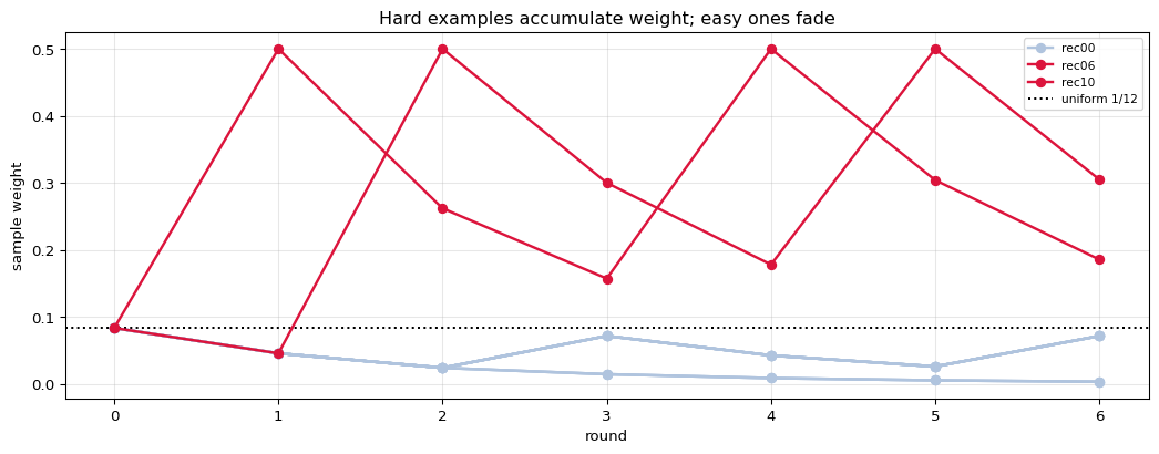
The weight vector is AdaBoost's memory. It says "here is what the ensemble still gets wrong", and the next weak learner is fitted to that, not to the raw data.
Notice what falls out of the reweighting: after each round the new stump's weighted error on the updated weights is exactly 0.5. The reweighting makes the previous learner useless on the new distribution — forcing the next one to find something different.
round    eps of THIS stump    eps of the PREVIOUS stump on new weights
------------------------------------------------------------------------
     1             0.083333
     2             0.045455                                    0.500000
     3             0.166667                                    0.500000
     4             0.157143                                    0.500000
------------------------------------------------------------------------

The right column sits at 0.5 - a coin flip. Each round deliberately
erases the previous learner's advantage, which is why the ensemble keeps
acquiring new information instead of repeating itself.

after 6 rounds the heaviest samples are: ['rec06', 'rec10', 'rec04']
   weights: [0.305  0.1855 0.0714]   (uniform would be 0.0833)

Those are the recordings that sit closest to the boundary - the same
ones the SVM walkthrough would call support vectors, arrived at by a
completely different route.
4. The Ensemble Prediction
$$F(x) = \sum_m \alpha_m h_m(x), \qquad \hat{y} = \operatorname{sign} F(x)$$
The magnitude of $F$ is a confidence: the margin. A point with $y F(x) \gg 0$ is correctly and confidently classified.
the 6-stump ensemble, evaluated on every recording

    id       a1h1       a2h2       a3h3       a4h4       a5h5       a6h6       F(x)   pred     y    margin
----------------------------------------------------------------------------------------------------------
 rec00    -1.1989    -1.5223     0.8047    -0.8398    -0.7651     0.7568    -2.7646     -1    -1    2.7646
 rec01    -1.1989    -1.5223     0.8047    -0.8398    -0.7651     0.7568    -2.7646     -1    -1    2.7646
 rec02     1.1989     1.5223     0.8047     0.8398     0.7651     0.7568     5.8876      1     1    5.8876
 rec03     1.1989     1.5223     0.8047     0.8398     0.7651     0.7568     5.8876      1     1    5.8876
 rec04    -1.1989    -1.5223     0.8047    -0.8398    -0.7651     0.7568    -2.7646     -1    -1    2.7646
 rec05     1.1989     1.5223    -0.8047     0.8398     0.7651    -0.7568     2.7646      1     1    2.7646
 rec06     1.1989    -1.5223     0.8047     0.8398    -0.7651     0.7568     1.3129      1     1    1.3129
 rec07     1.1989     1.5223    -0.8047     0.8398     0.7651    -0.7568     2.7646      1     1    2.7646
 rec08    -1.1989    -1.5223     0.8047    -0.8398    -0.7651     0.7568    -2.7646     -1    -1    2.7646
 rec09     1.1989     1.5223    -0.8047     0.8398     0.7651    -0.7568     2.7646      1     1    2.7646
 rec10     1.1989    -1.5223    -0.8047     0.8398    -0.7651    -0.7568    -1.8101     -1    -1    1.8101
 rec11     1.1989     1.5223     0.8047     0.8398     0.7651     0.7568     5.8876      1     1    5.8876
----------------------------------------------------------------------------------------------------------

ensemble accuracy: 1.0000   (12/12)
single best stump : 0.9167


how accuracy and margin evolve

 rounds   train accuracy    min margin     exp loss
--------------------------------------------------
      1           0.9167       -1.1989     0.552771
      2           0.9167       -0.3233     0.230283
      3           1.0000        0.4814     0.171643
      4           1.0000        0.2882     0.124934
      5           1.0000        0.5561     0.095570
      6           1.0000        1.3129     0.073500
--------------------------------------------------

Even after training accuracy reaches its ceiling, the MARGIN keeps
improving and the exponential loss keeps falling. That is the classic
AdaBoost observation: test error often continues to fall after training
error hits zero, because the ensemble is still growing more confident.
5. Why the Exponential Loss
AdaBoost is not a heuristic. It is exactly forward stagewise additive modelling under the exponential loss:
$$\mathcal{L} = \sum_i \exp\big(-y_i F(x_i)\big)$$
At each round it adds the term $\alpha_m h_m$ that most reduces that loss, holding everything already added fixed — and the $\alpha$ formula above is the exact minimiser. That connection is what places AdaBoost in the same family as gradient boosting: same additive structure, different loss.
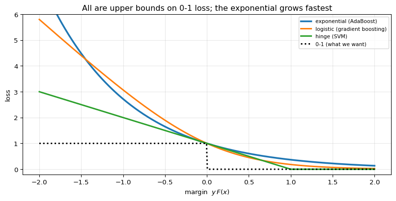
The exponential loss also explains AdaBoost's known weakness. It penalises a misclassified point exponentially in its margin, so a mislabelled example can dominate the weights entirely. AdaBoost is famously sensitive to label noise, and this is why.
margin    exponential     logistic     ratio
--------------------------------------------
     0.0         1.0000       1.0000      1.00x
    -0.5         1.6487       1.8946      0.87x
    -1.0         2.7183       3.0685      0.89x
    -2.0         7.3891       5.7970      1.27x
    -3.0        20.0855       8.6597      2.32x
    -4.0        54.5982      11.5420      4.73x
--------------------------------------------

At a margin of -4 the exponential loss is 54.6 while logistic is 11.5.
One badly mislabelled point can therefore soak up almost all the weight.


label noise: flip one label and watch

 round    weight on the flipped point    share of total
--------------------------------------------------------
     1                       0.250000            25.0%
     2                       0.178571            17.9%
     4                       0.286458            28.6%
     6                       0.289474            28.9%
     8                       0.373679            37.4%
--------------------------------------------------------

One mislabelled recording ends up carrying 37% of all the weight.
Every subsequent weak learner is fitted mainly to an error in the data.

This is why gradient boosting with a logistic loss largely replaced
AdaBoost in practice - same additive idea, a loss that does not
over-react.
6. Checking Against scikit-learn
scikit-learn implements SAMME, the multi-class generalisation, which reduces to the
binary formulas above when there are two classes. With
estimator=DecisionTreeClassifier(max_depth=1) it uses exactly the stumps used here.
(As of scikit-learn 1.8 the algorithm argument is gone — SAMME is the only option.)
round     our alpha    sklearn alpha     ratio
----------------------------------------------
     1      1.198948         2.397895    2.000x
     2      1.522261         3.044522    2.000x
     3      0.804719         1.609438    2.000x
     4      0.839821         1.679642    2.000x
     5      0.765094         1.530189    2.000x
     6      0.756778         1.513556    2.000x
----------------------------------------------

sklearn's SAMME uses alpha = ln((1-eps)/eps) + ln(K-1), which for K = 2
classes is ln((1-eps)/eps) - exactly TWICE our 0.5*ln(...).
The factor of 2 cancels in sign(F), so the predictions are identical:

   every ratio is 2: True

   our predictions     : [-1 -1  1  1 -1  1  1  1 -1  1 -1  1]
   sklearn predictions : [-1 -1  1  1 -1  1  1  1 -1  1 -1  1]
   MATCH: True
   accuracy ours 1.0000  sklearn 1.0000   MATCH: True


stumps chosen, ours vs sklearn

 round                                ours                             sklearn
------------------------------------------------------------------------------
     1                line_length <= 25.00                  spike_rate <= 3.55
     2                  spike_rate <= 3.55                line_length <= 25.00
     3                line_length <= 43.50                line_length <= 43.50
     4                line_length <= 25.00                  spike_rate <= 3.55
     5                  spike_rate <= 3.55                line_length <= 25.00
     6                line_length <= 43.50                line_length <= 43.50
------------------------------------------------------------------------------


staged accuracy

 rounds       ours    sklearn    match
------------------------------------
      1     0.9167     0.9167     True
      2     0.9167     0.9167     True
      3     1.0000     1.0000     True
      4     1.0000     1.0000     True
      5     1.0000     1.0000     True
      6     1.0000     1.0000     True
------------------------------------
7. Summary
| Step | Formula |
|---|---|
| Weighted error | $\varepsilon_m = \sum_i w_i\,\mathbb{1}[h_m(x_i)\ne y_i]$ |
| Vote | $\alpha_m = \tfrac12\ln\frac{1-\varepsilon_m}{\varepsilon_m}$ |
| Reweight | $w_i \leftarrow w_i e^{-\alpha_m y_i h_m(x_i)}$, renormalise |
| Predict | $\operatorname{sign}\sum_m \alpha_m h_m(x)$ |
| Implied loss | $\sum_i e^{-y_iF(x_i)}$ |
The one idea: make the data harder instead of the model bigger. Each round re-describes the problem so that what remains unsolved is what matters, and a sequence of one-question models becomes a strong classifier.
How it relates to the rest of the series: AdaBoost and gradient boosting are the same additive scheme, $F_m = F_{m-1} + \alpha_m h_m$. AdaBoost reaches it through reweighting under exponential loss; XGBoost reaches it by fitting gradients of an arbitrary loss. Recognising AdaBoost as "gradient boosting with the exponential loss" is what unified the two, and gradient boosting won because any loss became usable.
Its known weakness, demonstrated above: the exponential loss reacts so strongly to large negative margins that a single mislabelled point can absorb most of the weight. On noisy labels, prefer a logistic loss.
What is deliberately left out: SAMME.R (which uses probabilities rather than hard votes), AdaBoost for regression, the margin-theory explanation of why test error keeps falling after training error reaches zero, and the use of deeper base learners.