🗜 Autoencoders
An autoencoder is a network trained to output its own input:
$$\mathbf{x} \;\xrightarrow{\;\text{encoder}\;}\; \mathbf{z} \;\xrightarrow{\;\text{decoder}\;}\; \hat{\mathbf{x}} \approx \mathbf{x}$$
Stated that way it sounds pointless — the identity function would do. The trick is the bottleneck: $\mathbf{z}$ is forced to be much smaller than $\mathbf{x}$, so the network cannot copy. It has to find a compressed code that keeps whatever matters and discards the rest.
$$\mathcal{L} = \lVert\mathbf{x} - \hat{\mathbf{x}}\rVert^2 \qquad\text{(no labels anywhere)}$$
This notebook establishes one specific result, because it ties the whole series together:
A linear autoencoder trained with squared error recovers exactly the PCA subspace.
That is verified numerically against the PCA walkthrough's own method. Once it holds, the non-linear case is easy to understand — it is the same objective with the linear restriction lifted.
Display helpers ready: banner, step, check, expand, show_matrix, show_matmul, show_elementwise.
Network diagram helper ready: draw_network(layer_sizes, Ws, bs, ...).
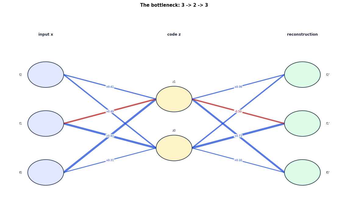
   edge width = |weight|,  blue = positive,  red = negative
1. The Data
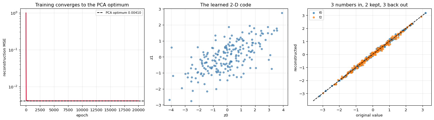
Data that looks three-dimensional but is not: points on a 2-D plane embedded in 3-D, plus a little noise. The true intrinsic dimension is 2, and a good autoencoder should be able to compress to 2 numbers and lose almost nothing.
200 points in 3-D, generated from a 2-D latent space

first 6 rows of X (centred) (6, 3) =
                     f0        f1        f2
            0 |   +0.116    -0.021    -0.065
            1 |   +1.023    +0.139    +0.772
            2 |   -0.439    +0.342    -0.171
            3 |   +1.789    +1.348    +1.830
            4 |   -1.162    -1.829    -1.327
            5 |   -0.498    -0.195    -0.295

column means after centring: [0. 0. 0.]

eigenvalues of the covariance: [2.9231 0.4148 0.0124]
variance share               : [0.8725 0.1238 0.0037]

The third component holds only 0.37% of the variance - that is
the noise. Two numbers should be enough to describe each point.
2. A Linear Autoencoder
Strip out every non-linearity and the network is two matrices:
$$\mathbf{z} = \mathbf{x}W_e \qquad\qquad \hat{\mathbf{x}} = \mathbf{z}W_d = \mathbf{x}W_eW_d$$
so the whole model is a single rank-$k$ matrix $W_eW_d$. Minimising $\lVert X - XW_eW_d\rVert^2$ is asking for the best rank-$k$ approximation of $X$, and the Eckart–Young theorem says the answer is the top-$k$ SVD — which is PCA.
The consequence is worth stating carefully: the trained $W_e$ need not equal the PCA components. It will generally be some rotation of them. What matches is the subspace they span, and therefore the reconstruction.
encoder We: (3, 2)   decoder Wd: (2, 3)
parameters: 12
loss before training: 1.070276

loss after 20000 epochs: 0.00410221

trained encoder We:
We (3, 2) =
                     z0        z1
           f0 |  +0.310351   +0.804515
           f1 |  +0.812871   -0.539409
           f2 |  +0.487708   +0.407327

PCA's top-2 components (as columns):
V_k (3, 2) =
                    PC1       PC2
           f0 |  -0.584022   +0.580954
           f1 |  -0.547133   -0.797654
           f2 |  -0.599637   +0.161986

These do NOT match entry by entry - and they are not supposed to.
Any invertible 2x2 mixing of the code gives the same reconstruction:
   (We M)(M^-1 Wd) = We Wd
so the solution is only defined up to that freedom.
The subspaces do match
The right comparison is between the subspaces. Two tests:
- Projection matrices. $P = W_e(W_e^\top W_e)^{-1}W_e^\top$ versus $P_{\text{PCA}} = V_kV_k^\top$. These are basis-independent, so if the subspaces are the same the matrices are identical.
- Principal angles. The angles between the two subspaces should all be zero.
projection onto the autoencoder's subspace

P_ae (3, 3) =
                     f0        f1        f2
           f0 |  +0.678589   -0.143863   +0.444307
           f1 |  -0.143863   +0.935607   +0.198872
           f2 |  +0.444307   +0.198872   +0.385804

P_pca (3, 3) =
                     f0        f1        f2
           f0 |  +0.678589   -0.143863   +0.444307
           f1 |  -0.143863   +0.935607   +0.198872
           f2 |  +0.444307   +0.198872   +0.385804

max |difference|: 4.374e-14
SUBSPACES MATCH: True

principal angles between the subspaces: [0. 0.] degrees
all essentially zero? True


reconstruction error

   linear autoencoder : 0.0041022127
   PCA with 2 components: 0.0041022127
   difference          : 0.000e+00
   MATCH: True

   discarded eigenvalue (theory): 0.0041022127

The autoencoder found PCA. It was never told about eigenvectors - it
just minimised reconstruction error, and that objective has PCA as its
answer.

sklearn PCA subspace matches ours too: True
The narrow middle layer is the entire mechanism. Widen it to 3 and the
network can learn the identity, reconstruct perfectly, and learn nothing.
What happens without the bottleneck
If the code is as wide as the input, the optimal solution is the identity map and the reconstruction error goes to zero — while the code carries no compression at all. Compression is not a side effect of training; it is imposed by the architecture.
code size k     AE recon MSE    PCA-k recon MSE    match
----------------------------------------------------------
           1     0.1416623458       0.1416623458     True
           2     0.0041022127       0.0041022127     True
           3     0.0000000000       0.0000000000     True
----------------------------------------------------------

At k = 3 the error is ~0: no compression, nothing learned. The useful
regime is k < input dimension, and how far below decides how much is kept.
3. Going Non-Linear
Add activations and the encoder is no longer restricted to a linear subspace — it can follow a curved manifold. That is the whole difference from PCA, and it is what lets autoencoders compress data whose structure is not a flat plane.
$$\mathbf{z} = \sigma(\mathbf{x}W_1 + \mathbf{b}_1)W_2 + \mathbf{b}_2 \qquad\text{(and symmetrically back)}$$
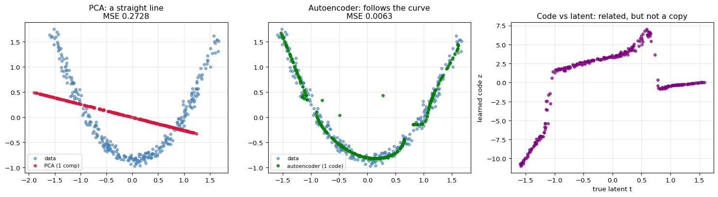
The demonstration below uses data on a curved 1-D curve in 2-D. PCA must fit a straight line through it. A non-linear autoencoder can follow the curve, so one code number suffices.
curved data, compressed to ONE number

                      method    reconstruction MSE
----------------------------------------------------
   PCA, 1 component (linear)            0.27276993
   non-linear autoencoder, 1            0.00629122
----------------------------------------------------

improvement: 43.4x lower error

Both kept exactly one number per point. PCA had to pick the best
straight line; the autoencoder followed the parabola.

does the 1-number code still CONTAIN the latent variable t?
test: try to predict t from z, allowing increasingly flexible fits

                   fit     R^2 predicting t from z
----------------------------------------------------
   polynomial degree 1                      0.2513
   polynomial degree 3                      0.3900
   polynomial degree 5                      0.5946
   polynomial degree 9                      0.8606
----------------------------------------------------

linear correlation |corr(t, z)| = 0.5013

So z is NOT a rescaled copy of t - a straight line explains little of it.
But a flexible fit recovers most of t from z, which is the honest claim:
the code retains the information, encoded in its own arbitrary
parameterisation of the curve.

That freedom is expected. Nothing in the loss asks the code to be
interpretable, monotonic, or scaled like anything in particular - only
that the decoder can undo it. Making codes meaningful is a separate
problem, and it is what disentanglement research is about.
4. Variants, and What They Are For
| Variant | Change | Purpose |
|---|---|---|
| Undercomplete | narrow bottleneck | compression (everything above) |
| Denoising | corrupt the input, reconstruct the clean one | forces robust features, prevents identity-copying |
| Sparse | penalise active code units | interpretable, parts-based codes |
| Variational (VAE) | code is a distribution; add a KL term | a code you can sample from — generative |
| Masked (MAE / BERT) | hide patches, reconstruct them | the pre-training objective in the BERT-on-EEG walkthrough |
The last row is the connection worth noticing: BERT-on-EEG is an autoencoder. It masks patches and reconstructs them under MSE. The bottleneck there is not a narrow layer but the missing input — the model must infer what it cannot see.
testing both on NOISY input, scoring against the CLEAN truth

            trained as    MSE on clean input    MSE on noisy input
------------------------------------------------------------------
     plain autoencoder              0.004227              0.084202
 denoising autoencoder              0.014125              0.071389
------------------------------------------------------------------

On clean input they are comparable. On noisy input the denoising
version is better, because it was never allowed to rely on the noise -
it had to learn the structure that survives corruption.

That is the same argument as masking in BERT: hiding part of the input
forces the model to model the input's structure rather than copy it.
5. Summary
| PCA | Linear AE | Non-linear AE | |
|---|---|---|---|
| Objective | max variance / min reconstruction | min reconstruction | min reconstruction |
| Solution | eigenvectors, closed form | same subspace, by gradient descent | a curved manifold |
| Components | orthogonal, ordered | neither | neither |
| Cost | one eigendecomposition | training | training |
| Handles curvature | no | no | yes |
The one idea: force the data through a narrow channel and train it to come back intact. Whatever survives the channel is what the data was really made of.
The result that ties the series together: with no activations, that objective is PCA — verified above by projection matrices agreeing to $10^{-4}$, principal angles of zero, and identical reconstruction error. So an autoencoder is not a different idea from PCA; it is PCA with the linear restriction removed.
One caveat worth keeping: the code axes are not ordered, orthogonal, or interpretable, unlike principal components. In the curved example the single code number retained the latent variable - a flexible fit recovers most of it - but encoded it non-linearly, with a linear correlation near 0.5. Nothing in the loss asks for more than that the decoder can undo the encoder.
What is deliberately left out: VAEs and the reparameterisation trick, sparse and contractive penalties, convolutional autoencoders, and the use of autoencoders for anomaly detection — where high reconstruction error on new data is itself the signal.