🐱 CatBoost
CatBoost uses the same objective as XGBoost and LightGBM — the leaf weight is still $w^{*} = -G/(H+\lambda)$. Its three distinctive ideas are all about leakage: places where a model accidentally uses information it would not have at prediction time.
| Idea | The leak it closes |
|---|---|
| Ordered target statistics | encoding a category with its own row's target |
| Ordered boosting | computing a residual with a model that already saw that row |
| Oblivious trees | (not leakage) one split per level — fast, and heavily regularised |
The first two are subtle and cost accuracy when ignored on small data. The third changes
what a tree even looks like. All three are worked through below, and the final tree is
verified leaf-for-leaf against the real catboost.
Display helpers ready: banner, step, check, expand, show_matrix, show_matmul, show_elementwise.
Tree diagram helper ready: draw_tree(root, title).
1. The Data
The same 12 EEG recordings, but now the categorical column matters: region is one
of frontal, temporal, occipital. Categories cannot be compared with $\le$, so a
tree cannot split on them directly — they must first be turned into numbers.
That conversion is where CatBoost's first idea lives.
12 recordings x 3 features

    id      region   line_length    spike_rate           age   y_class    y_reg
-------------------------------------------------------------------------------
 rec00     frontal          12.0           0.5          24.0         0      0.2
 rec01    temporal          15.0           1.2          31.0         0      0.5
 rec02    temporal          42.0           6.8          58.0         1      6.4
 rec03   occipital          38.0           5.1          47.0         1      4.8
 rec04     frontal          11.0           0.3          19.0         0      0.1
 rec05    temporal          55.0           8.2          63.0         1      9.1
 rec06   occipital          40.0           1.9          35.0         1      3.5
 rec07    temporal          47.0           7.4          52.0         1      7.2
 rec08     frontal          14.0           0.8          28.0         0      0.3
 rec09   occipital          51.0           6.1          60.0         1      6.9
 rec10     frontal          45.0           2.4          41.0         0      1.6
 rec11    temporal          35.0           4.7          30.0         1      4.1
-------------------------------------------------------------------------------

class balance: 5 negative, 7 positive
y_reg mean = 3.7250, std = 3.0518
category membership

   frontal (4 rows): ['rec00', 'rec04', 'rec08', 'rec10']
            y_class = [0 0 0 0]   mean = 0.0000
  temporal (5 rows): ['rec01', 'rec02', 'rec05', 'rec07', 'rec11']
            y_class = [0 1 1 1 1]   mean = 0.8000
 occipital (3 rows): ['rec03', 'rec06', 'rec09']
            y_class = [1 1 1]   mean = 1.0000

global mean of y_class (the 'prior') = 0.583333
2. The Leak in Naive Target Encoding
The obvious way to turn a category into a number is to replace it with the mean target of that category (target encoding, or "greedy TS"):
$$\hat x_i = \frac{\sum_{j} \mathbb{1}[\,x_j = x_i\,]\, y_j}{\sum_{j} \mathbb{1}[\,x_j = x_i\,]}$$
The sum runs over all rows — including row $i$ itself. That is the leak: row $i$'s own label is baked into row $i$'s own feature.
The effect is worst for rare categories. For a category with a single member the encoding is that member's target, so the feature becomes a perfect copy of the answer — on training data only.
naive target encoding of 'region'

    id      region    y    encoded   includes own y?
----------------------------------------------------
 rec00     frontal    0     0.0000               YES
 rec01    temporal    0     0.8000               YES
 rec02    temporal    1     0.8000               YES
 rec03   occipital    1     1.0000               YES
 rec04     frontal    0     0.0000               YES
 rec05    temporal    1     0.8000               YES
 rec06   occipital    1     1.0000               YES
 rec07    temporal    1     0.8000               YES
 rec08     frontal    0     0.0000               YES
 rec09   occipital    1     1.0000               YES
 rec10     frontal    0     0.0000               YES
 rec11    temporal    1     0.8000               YES
----------------------------------------------------

correlation between the encoded feature and the target: 0.8519

Now the extreme case. Suppose one recording came from a region seen only once:
   rec06 is the only 'parietal' recording, y = 1
   its naive encoding = 1.0000
   equals its own label exactly: True

A tree splitting on that feature would separate this row perfectly during
training and learn nothing that transfers. At prediction time the row's label
is unknown, so the feature cannot be computed the same way at all.
3. Ordered Target Statistics
CatBoost's fix: fix a random permutation of the rows and pretend they arrive in that order. Encode each row using only the rows that came before it, smoothed toward a prior $P$ with weight $a$:
$$\hat x_{\sigma(i)} = \frac{\displaystyle\sum_{j < i} \mathbb{1}[\,x_{\sigma(j)} = x_{\sigma(i)}\,]\, y_{\sigma(j)} \;+\; a\,P} {\displaystyle\sum_{j < i} \mathbb{1}[\,x_{\sigma(j)} = x_{\sigma(i)}\,] \;+\; a}$$
Two things fall out at once:
- Row $i$'s own target never enters its own encoding — the leak is closed by construction.
- The first occurrence of any category has an empty history, so it falls back to the prior $P$ — which is exactly the right behaviour for an unseen category at prediction time.
$P$ is normally the global mean of $y$, and $a > 0$ keeps early, low-count estimates from being wild.
prior P = 0.583333,  smoothing a = 1.0

permutation (arrival order): ['rec01', 'rec00', 'rec08', 'rec02', 'rec10', 'rec09', 'rec07', 'rec06', 'rec04', 'rec03', 'rec05', 'rec11']

 pos      id      region    y   count before   sum y before    encoded
----------------------------------------------------------------------
   0   rec01    temporal    0              0            0.0     0.5833  <- no history, falls back to prior
   1   rec00     frontal    0              0            0.0     0.5833  <- no history, falls back to prior
   2   rec08     frontal    0              1            0.0     0.2917
   3   rec02    temporal    1              1            0.0     0.2917
   4   rec10     frontal    0              2            0.0     0.1944
   5   rec09   occipital    1              0            0.0     0.5833  <- no history, falls back to prior
   6   rec07    temporal    1              2            1.0     0.5278
   7   rec06   occipital    1              1            1.0     0.7917
   8   rec04     frontal    0              3            0.0     0.1458
   9   rec03   occipital    1              2            2.0     0.8611
  10   rec05    temporal    1              3            2.0     0.6458
  11   rec11    temporal    1              4            3.0     0.7167
----------------------------------------------------------------------

worked example, position 5:
   row rec09, region 'occipital'
   rows before it in this permutation: ['rec01', 'rec00', 'rec08', 'rec02', 'rec10']
   of those, same region             : []  (y = [])
   encoded = (sum + a*P) / (count + a)
           = (0.0 + 1.0*0.5833) / (0 + 1.0)
           = 0.5833 / 1.0 = 0.583333
   note that y[rec09] = 1 was NOT used.


correlation with target, naive  : +0.8519
correlation with target, ordered: +0.5950

The ordered encoding is less correlated with the target - and that is the
point. The extra correlation in the naive version was leakage, not signal.
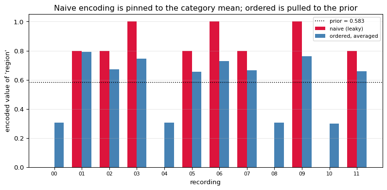
Averaging over permutations
A single permutation is noisy: the row that happens to arrive first always gets the prior, whatever its category. CatBoost therefore uses several independent permutations and averages the resulting statistics, which keeps the no-leak property while cutting the variance.
id      region    y     naive    1 perm   avg of 200      std
-----------------------------------------------------------------
 rec00     frontal    0    0.0000    0.5833       0.3048   0.1733
 rec01    temporal    0    0.8000    0.5833       0.7916   0.1300
 rec02    temporal    1    0.8000    0.2917       0.6713   0.1386
 rec03   occipital    1    1.0000    0.8611       0.7455   0.1173
 rec04     frontal    0    0.0000    0.1458       0.3055   0.1690
 rec05    temporal    1    0.8000    0.6458       0.6567   0.1522
 rec06   occipital    1    1.0000    0.7917       0.7295   0.1200
 rec07    temporal    1    0.8000    0.5278       0.6642   0.1495
 rec08     frontal    0    0.0000    0.2917       0.3050   0.1723
 rec09   occipital    1    1.0000    0.5833       0.7611   0.1147
 rec10     frontal    0    0.0000    0.1944       0.2999   0.1641
 rec11    temporal    1    0.8000    0.7167       0.6578   0.1367
-----------------------------------------------------------------

spread across permutations for a single row (rec00):
   min 0.1458, max 0.5833, mean 0.3048

no permutation ever lets a row see its own target, so the average
is still leak-free - it is just a lower-variance estimate.
4. Ordered Boosting
The same leak appears a second time, and it is easier to miss.
In ordinary gradient boosting the residual for row $i$ is computed from a model that was trained on row $i$. So the residual is optimistically small — the model has already partly memorised that row. Bias accumulates over rounds; CatBoost's authors call it prediction shift.
Ordered boosting closes it with the same trick: keep a set of models $M_0, M_1, \dots$ where $M_k$ has only ever seen the first $k$ rows of the permutation, and compute row $i$'s gradient with $M_{i-1}$:
$$g_i = \frac{\partial\, l\big(y_i,\; M_{i-1}(x_i)\big)}{\partial \hat y}$$
The row being scored was never in the training set of the model scoring it.
Switching to the regression target y_reg for the boosting sections.

 pos      id        y   model saw row?   plain resid   ordered resid
--------------------------------------------------------------------
   0   rec03     4.80              YES        1.0750          1.0750
   1   rec02     6.40              YES        2.6750          1.6000
   2   rec06     3.50              YES       -0.2250         -2.1000
   3   rec00     0.20              YES       -3.5250         -4.7000
   4   rec07     7.20              YES        3.4750          3.4750
   5   rec11     4.10              YES        0.3750         -0.3200
   6   rec09     6.90              YES        3.1750          2.5333
   7   rec08     0.30              YES       -3.4250         -4.4286
   8   rec05     9.10              YES        5.3750          4.9250
   9   rec10     1.60              YES       -2.1250         -3.1222
  10   rec04     0.10              YES       -3.6250         -4.3100
  11   rec01     0.50              YES       -3.2250         -3.5182
--------------------------------------------------------------------

mean |residual|, plain  : 2.6917
mean |residual|, ordered: 3.0089

The ordered residuals are LARGER. That is the honest number - the plain
ones look smaller only because each row helped fit the model that scored it.

CatBoost pays for this with bookkeeping: conceptually O(n) models per
permutation. In practice it maintains them on a tree of prefixes so the
cost stays close to ordinary boosting.
5. Oblivious Trees
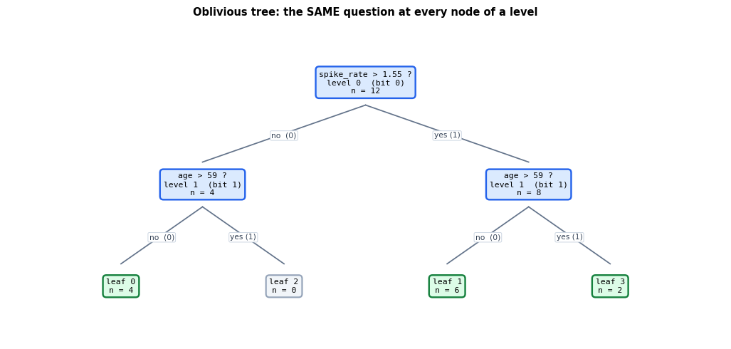
CatBoost's trees are oblivious (also called symmetric): every node at the same depth uses the same feature and the same threshold.
A normal depth-$d$ tree chooses up to $2^d - 1$ independent splits. An oblivious tree of depth $d$ chooses exactly $d$.
That is a severe restriction, and it buys two things:
Regularisation. With far fewer split decisions the tree cannot chase noise, which suits boosting where each tree is meant to be weak.
Inference speed. Because the same comparison applies to every row at a given depth, the leaf index is just $d$ bits packed into an integer:
$$\text{leaf}(x) \;=\; \sum_{k=0}^{d-1} 2^{k}\,\mathbb{1}\big[x_{f_k} > t_k\big]$$
No branching, no pointer chasing — $d$ comparisons and one array lookup, fully vectorisable.
depth 1:  normal tree picks up to   1 splits,  oblivious picks  1   ->  both have   2 leaves
depth 2:  normal tree picks up to   3 splits,  oblivious picks  2   ->  both have   4 leaves
depth 3:  normal tree picks up to   7 splits,  oblivious picks  3   ->  both have   8 leaves
depth 4:  normal tree picks up to  15 splits,  oblivious picks  4   ->  both have  16 leaves
depth 6:  normal tree picks up to  63 splits,  oblivious picks  6   ->  both have  64 leaves
depth 8:  normal tree picks up to 255 splits,  oblivious picks  8   ->  both have 256 leaves


An oblivious tree of depth 2, using CatBoost's own two splits:

   level 0: spike_rate > 1.55   ->  bit 0 (worth 1)
   level 1: age > 59.0   ->  bit 1 (worth 2)

    id    spike_rate>1.55           age>59.0    bits   leaf
------------------------------------------------------------
 rec00           no (0.5)            no (24)      00      0
 rec01           no (1.2)            no (31)      00      0
 rec02          yes (6.8)            no (58)      01      1
 rec03          yes (5.1)            no (47)      01      1
 rec04           no (0.3)            no (19)      00      0
 rec05          yes (8.2)           yes (63)      11      3
 rec06          yes (1.9)            no (35)      01      1
 rec07          yes (7.4)            no (52)      01      1
 rec08           no (0.8)            no (28)      00      0
 rec09          yes (6.1)           yes (60)      11      3
 rec10          yes (2.4)            no (41)      01      1
 rec11          yes (4.7)            no (30)      01      1
------------------------------------------------------------

leaf occupancy: [4, 6, 0, 2]
   leaf 2 is EMPTY - no recording has spike_rate <= 1.55 AND age > 59.
   An oblivious tree cannot avoid such leaves: the same split is forced on
   every branch, whether or not it is useful there. That is the price.
The oblivious tree, drawn
Notice what is different from every other tree diagram in this series: both nodes at
depth 1 ask the identical question (age > 59). That is the whole meaning of
"oblivious" — the tree is a list of $d$ questions, not a branching structure of
$2^d - 1$ independent ones.
The leaf values shown are the ones computed in the next section and confirmed against the real library.
Both depth-1 boxes ask the same thing. A normal tree would be free to ask
two different questions there - an oblivious tree is not.

a normal depth-2 tree chooses up to 3 splits; this one chooses 2.
Fewer decisions means less capacity to chase noise, and it means the leaf
index is just the answer bits read as a binary number.
6. Checking Against the Real CatBoost
CatBoost is trained below with one tree of depth 2. Two things are then verified by hand:
- the leaf assignment from the bit arithmetic above, and
- the leaf values, from the same formula every model in this series uses:
$$\text{leaf value} \;=\; \eta \cdot \frac{\sum_{i \in \text{leaf}} (y_i - \hat y_i)}{n_{\text{leaf}} + \lambda}$$
catboost bias (starting prediction) = 3.725000   mean(y) = 3.725000   MATCH: True

catboost's splits, one per level:
   level 0: spike_rate > 1.550000
   level 1: age > 59.000000

our assumed splits matched: True

 leaf                          rows    n   cb weight    our value     catboost   match
--------------------------------------------------------------------------------------
    0      ['00', '01', '04', '08']    4           4    -0.828000    -0.828000    True
    1  ['02', '03', '06', '07', '10', '11']    6           6     0.225000     0.225000    True
    2                            []    0           0     0.000000     0.000000    True
    3                  ['05', '09']    2           2     0.855000     0.855000    True
--------------------------------------------------------------------------------------

leaf weights MATCH : True
leaf values MATCH  : True

worked example, leaf 0:
   rows ['rec00', 'rec01', 'rec04', 'rec08']
   y            = [0.2 0.5 0.1 0.3]
   y - bias     = [-3.525 -3.225 -3.625 -3.425]
   sum          = -13.800001
   / (n + l2)   = -13.800001 / (4 + 1.0) = -2.760000
   x eta        = 0.3 * -2.760000 = -0.828000
   catboost     = -0.828000
id        y   leaf        ours     catboost        diff
-----------------------------------------------------------
 rec00     0.20      0    2.897000     2.897000    3.19e-08
 rec01     0.50      0    2.897000     2.897000    3.19e-08
 rec02     6.40      1    3.950000     3.950000    9.96e-09
 rec03     4.80      1    3.950000     3.950000    9.96e-09
 rec04     0.10      0    2.897000     2.897000    3.19e-08
 rec05     9.10      3    4.580000     4.580000    8.17e-08
 rec06     3.50      1    3.950000     3.950000    9.96e-09
 rec07     7.20      1    3.950000     3.950000    9.96e-09
 rec08     0.30      0    2.897000     2.897000    3.19e-08
 rec09     6.90      3    4.580000     4.580000    8.17e-08
 rec10     1.60      1    3.950000     3.950000    9.96e-09
 rec11     4.10      1    3.950000     3.950000    9.96e-09
-----------------------------------------------------------

predictions MATCH catboost: True

MSE before: 9.313542
MSE after : 6.369570
One caveat, stated plainly
The leaf values above are reproduced exactly, because they follow the closed-form
formula. The choice of splits is not re-derived here: CatBoost quantises features
into borders with its own algorithm and adds a random component (random_strength)
before comparing candidates, so its two splits are not simply the greedy best two.
This walkthrough therefore takes CatBoost's splits as given and verifies everything downstream of them.
7. Summary
| Idea | Formula | Effect |
|---|---|---|
| Ordered target statistic | $\dfrac{\sum_{j<i}\mathbb{1}[x_j=x_i]y_j + aP}{\sum_{j<i}\mathbb{1}[x_j=x_i] + a}$ | category encoding never sees its own label |
| Prior fallback | first occurrence $\to P$ | matches unseen-category behaviour at inference |
| Ordered boosting | $g_i$ from $M_{i-1}$ | removes prediction shift |
| Oblivious tree | $\text{leaf} = \sum_k 2^k \mathbb{1}[x_{f_k} > t_k]$ | $d$ splits, $2^d$ leaves, branch-free inference |
| Leaf value | $\eta\,\dfrac{\sum (y_i - \hat y_i)}{n + \lambda}$ | identical to XGBoost |
The one idea: both of CatBoost's "ordered" mechanisms are the same insight applied twice — never let a row influence the number used to describe or score that row. It is the logic of a train/test split, pushed down to the level of the individual row.
When it matters most: small datasets and high-cardinality categorical features, which is exactly where naive target encoding leaks hardest.
What is deliberately left out: feature combinations (CatBoost builds categorical
crosses automatically), random_strength and the details of border selection, GPU
histogram computation, and the multi-permutation bookkeeping that makes ordered boosting
affordable.
The series in one table
| Model | What it contributes | Split rule |
|---|---|---|
| Decision Tree | the greedy split search itself | maximise Gini gain |
| Random Forest | variance reduction by averaging | same, on bootstrapped rows and random features |
| XGBoost | closed-form leaf and gain from a 2nd-order expansion | maximise $\frac{G^2}{H+\lambda}$ |
| LightGBM | the same math, a much faster search | histogram + leaf-wise |
| CatBoost | leak-free encoding and residuals | same math, oblivious structure |
Every one of them is the same greedy question — which split helps most? — with a different definition of "helps" and a different budget for finding out.