🖼 Convolutional Networks
A dense layer connects every input to every output. For a 100×100 image that is 10 000 inputs, so one hidden layer of 1 000 units needs ten million weights — and having learned to recognise something in the top-left corner, it would have learned nothing about the same thing in the bottom-right, because those are different weights entirely.
A convolution fixes both problems with one idea: use a small set of weights, and slide it across the whole input.
$$(\,I * K)[i,j] \;=\; \sum_{u}\sum_{v} I[i+u,\; j+v]\;K[u,v]$$
Two consequences follow, and they are the reason convolutional networks exist:
- Parameter sharing — the same 9 numbers are reused at every position, so cost stops scaling with input size.
- Translation equivariance — a pattern learned anywhere is detected everywhere, because it is literally the same detector being moved.
Everything below is worked out by hand on matrices small enough to print, then checked against PyTorch.
Display helpers ready: banner, step, check, expand, show_matrix, show_matmul, show_elementwise.
1. Convolution, One Position at a Time
Start with a 6×6 input and a 3×3 kernel. The kernel is placed over the top-left corner, the nine products are summed, and the result becomes one output pixel. Then the kernel slides one step right and it happens again.
The input below has a vertical edge: values jump from 1 to 8 between columns 2 and 3.
input I (6x6) - a bright region on the right, dark on the left

I (6, 6) =
            0 |    1.0     1.0     1.0     8.0     8.0     8.0
            1 |    1.0     1.0     1.0     8.0     8.0     8.0
            2 |    1.0     1.0     1.0     8.0     8.0     8.0
            3 |    1.0     1.0     1.0     8.0     8.0     8.0
            4 |    1.0     1.0     1.0     8.0     8.0     8.0
            5 |    1.0     1.0     1.0     8.0     8.0     8.0

kernel K (3x3) (3, 3) =
            0 |    1.0     0.0    -1.0
            1 |    1.0     0.0    -1.0
            2 |    1.0     0.0    -1.0

output size: (6 - 3)/1 + 1 = 4 x 4

output O (4, 4) =
            0 |      0.0     -21.0     -21.0       0.0
            1 |      0.0     -21.0     -21.0       0.0
            2 |      0.0     -21.0     -21.0       0.0
            3 |      0.0     -21.0     -21.0       0.0


position (0,0) written out in full:

patch = I[0:3, 0:3] (3, 3) =
            0 |    1.0     1.0     1.0
            1 |    1.0     1.0     1.0
            2 |    1.0     1.0     1.0

   O[0,0] = (1)*(+1) + (1)*(+0) + (1)*(-1) + (1)*(+1) + (1)*(+0)
          + (1)*(-1) + (1)*(+1) + (1)*(+0) + (1)*(-1)
          = 0.0
   from the array: 0.0   MATCH: True

   The patch is uniform (all 1s), and the kernel's weights sum to zero,
   so everything cancels. Flat regions produce nothing.


position (0,1) - now the patch straddles the edge:

patch = I[0:3, 1:4] (3, 3) =
            0 |    1.0     1.0     8.0
            1 |    1.0     1.0     8.0
            2 |    1.0     1.0     8.0

   O[0,1] = (1)*(+1) + (1)*(+0) + (8)*(-1) + (1)*(+1) + (1)*(+0)
          + (8)*(-1) + (1)*(+1) + (1)*(+0) + (8)*(-1)
          = -21.0

   The left column sees 1s, the right column sees 8s, and the kernel
   subtracts right from left: 3*(1) - 3*(8) = -21. The edge is found.
The kernel is the feature detector
A convolution does not "look for edges" because someone wrote edge-detection code. It computes a dot product between the kernel and each patch, so it responds most strongly to patches that look like the kernel. Change the nine numbers and you change what the layer detects.
In a trained network nobody chooses these numbers — they are learned by exactly the gradient descent from the Neural Network walkthrough.
input J - a vertical edge at column 4 and a horizontal edge at row 4

J (7, 7) =
            0 |   1.0    1.0    1.0    1.0    8.0    8.0    8.0
            1 |   1.0    1.0    1.0    1.0    8.0    8.0    8.0
            2 |   1.0    1.0    1.0    1.0    8.0    8.0    8.0
            3 |   1.0    1.0    1.0    1.0    8.0    8.0    8.0
            4 |   5.0    5.0    5.0    5.0    5.0    5.0    5.0
            5 |   5.0    5.0    5.0    5.0    5.0    5.0    5.0
            6 |   5.0    5.0    5.0    5.0    5.0    5.0    5.0


--- vertical edge ---   kernel sum = 0.00
K (3, 3) =
            0 |   1.00    0.00   -1.00
            1 |   1.00    0.00   -1.00
            2 |   1.00    0.00   -1.00

output (5, 5) =
            0 |    0.00     0.00   -21.00   -21.00     0.00
            1 |    0.00     0.00   -21.00   -21.00     0.00
            2 |    0.00     0.00   -14.00   -14.00     0.00
            3 |    0.00     0.00    -7.00    -7.00     0.00
            4 |    0.00     0.00     0.00     0.00     0.00


--- horizontal edge ---   kernel sum = 0.00
K (3, 3) =
            0 |   1.00    1.00    1.00
            1 |   0.00    0.00    0.00
            2 |  -1.00   -1.00   -1.00

output (5, 5) =
            0 |    0.00     0.00     0.00     0.00     0.00
            1 |    0.00     0.00     0.00     0.00     0.00
            2 |  -12.00   -12.00    -5.00     2.00     9.00
            3 |  -12.00   -12.00    -5.00     2.00     9.00
            4 |    0.00     0.00     0.00     0.00     0.00


--- blur (average) ---   kernel sum = 1.00
K (3, 3) =
            0 |   0.11    0.11    0.11
            1 |   0.11    0.11    0.11
            2 |   0.11    0.11    0.11

output (5, 5) =
            0 |    1.00     1.00     3.33     5.67     8.00
            1 |    1.00     1.00     3.33     5.67     8.00
            2 |    2.33     2.33     3.89     5.44     7.00
            3 |    3.67     3.67     4.44     5.22     6.00
            4 |    5.00     5.00     5.00     5.00     5.00


--- sharpen ---   kernel sum = 1.00
K (3, 3) =
            0 |   0.00   -1.00    0.00
            1 |  -1.00    5.00   -1.00
            2 |   0.00   -1.00    0.00

output (5, 5) =
            0 |    1.00     1.00    -6.00    15.00     8.00
            1 |    1.00     1.00    -6.00    15.00     8.00
            2 |   -3.00    -3.00   -10.00    18.00    11.00
            3 |    9.00     9.00     9.00     2.00     2.00
            4 |    5.00     5.00     5.00     5.00     5.00


--- identity ---   kernel sum = 1.00
K (3, 3) =
            0 |   0.00    0.00    0.00
            1 |   0.00    1.00    0.00
            2 |   0.00    0.00    0.00

output (5, 5) =
            0 |    1.00     1.00     1.00     8.00     8.00
            1 |    1.00     1.00     1.00     8.00     8.00
            2 |    1.00     1.00     1.00     8.00     8.00
            3 |    5.00     5.00     5.00     5.00     5.00
            4 |    5.00     5.00     5.00     5.00     5.00


why the kernel SUM matters:
   sums to 0  -> flat areas give 0; the kernel measures CHANGE (edges)
   sums to 1  -> flat areas are preserved; the kernel measures INTENSITY

   vertical edge kernel sums to 0  -> flat region output: 0.0
   blur kernel sums to 1  -> flat region output: 1.0
Blue and red are opposite signs. The vertical-edge kernel lights up only
along the vertical boundary, the horizontal one only along the horizontal
boundary, and the identity kernel reproduces the input unchanged.

2. Stride, Padding, and Output Size
Three settings control the output shape:
$$\text{out} = \left\lfloor \frac{\text{in} + 2p - k}{s} \right\rfloor + 1$$
- kernel size $k$ — how much context each output sees
- stride $s$ — how far the kernel jumps; $s = 2$ halves the resolution
- padding $p$ — zeros added around the border
Padding exists because without it every convolution shrinks the input, and border pixels
are visited far less often than middle ones. padding = (k-1)/2 keeps the size fixed —
"same" padding.
in    k   stride   pad                     formula    out   actual   match
----------------------------------------------------------------------------
   6    3        1     0         (6 + 2*0 - 3)/1 + 1      4        4    True
   6    3        2     0         (6 + 2*0 - 3)/2 + 1      2        2    True
   6    3        1     1         (6 + 2*1 - 3)/1 + 1      6        6    True
   7    3        1     1         (7 + 2*1 - 3)/1 + 1      7        7    True
   7    3        2     1         (7 + 2*1 - 3)/2 + 1      4        4    True
   8    5        1     0         (8 + 2*0 - 5)/1 + 1      4        4    True
   8    5        1     2         (8 + 2*2 - 5)/1 + 1      8        8    True
   8    3        3     0         (8 + 2*0 - 3)/3 + 1      2        2    True
----------------------------------------------------------------------------

'same' padding keeps the size: for k = 3, p = 1; for k = 5, p = 2

   input 5x5, k=3, p=0 -> (3, 3)   (shrunk)
   input 5x5, k=3, p=1 -> (5, 5)   (same)


how often is each pixel used, without padding? (3x3 kernel on 5x5)

times each input pixel is read (5, 5) =
            0 |     1      2      3      2      1
            1 |     2      4      6      4      2
            2 |     3      6      9      6      3
            3 |     2      4      6      4      2
            4 |     1      2      3      2      1

   corner pixel: 1 time,  centre pixel: 9 times
   Without padding the borders are systematically under-weighted.


stride 2 - the kernel jumps two positions, halving resolution:

input 6x6 (6, 6) =
            0 |     0      1      2      3      4      5
            1 |     6      7      8      9     10     11
            2 |    12     13     14     15     16     17
            3 |    18     19     20     21     22     23
            4 |    24     25     26     27     28     29
            5 |    30     31     32     33     34     35

identity kernel, stride 2 (2, 2) =
            0 |      7       9
            1 |     19      21

   It kept rows/cols 1, 3 and skipped the rest - downsampling, and the
   skipped information is simply gone.
3. Channels and Filters
Real inputs have depth: an RGB image is 3 channels, a multi-channel EEG recording is one channel per electrode. And one kernel detects only one pattern, so a layer uses many.
$$\text{one filter: } \;\; O[i,j] = \sum_{c=1}^{C_{in}}\sum_{u}\sum_{v} I[c,\,i+u,\,j+v]\;K[c,u,v] \;+\; b$$
Two things to get right:
- A filter spans all input channels and sums over them, producing one output map.
- A layer has $C_{out}$ such filters, so the weight tensor is $(C_{out}, C_{in}, k, k)$ and the output has $C_{out}$ channels.
input: 2 channels of 5x5

channel 0 (5, 5) =
            0 |   1.0    1.0    1.0    6.0    6.0
            1 |   1.0    1.0    1.0    6.0    6.0
            2 |   1.0    1.0    1.0    6.0    6.0
            3 |   1.0    1.0    1.0    6.0    6.0
            4 |   1.0    1.0    1.0    6.0    6.0

channel 1 (5, 5) =
            0 |   2.0    2.0    2.0    2.0    2.0
            1 |   2.0    2.0    2.0    2.0    2.0
            2 |   9.0    9.0    9.0    9.0    9.0
            3 |   9.0    9.0    9.0    9.0    9.0
            4 |   9.0    9.0    9.0    9.0    9.0

weights W: (3, 2, 3, 3)  = (out_channels, in_channels, k, k)
bias b   : (3,)
output   : (3, 3, 3)  = (3 feature maps of 3x3)

filter 0, spanning both input channels:

W[0, channel 0] (3, 3) =
            0 | +0.0629  -0.0661  +0.3202
            1 | +0.0525  -0.2678  +0.1808
            2 | +0.6520  +0.4735  -0.3519

W[0, channel 1] (3, 3) =
            0 | -0.6327  -0.3116  +0.0207
            1 | -1.1625  -0.1094  -0.6230
            2 | -0.3661  -0.2721  -0.1582


output[0, 0, 0] computed in full:

   contribution from channel 0: sum(patch0 * W[0,0]) = +1.056110
   contribution from channel 1: sum(patch1 * W[0,1]) = -12.804823
   + bias b[0] = -0.128836
   total = +1.056110 -12.804823 -0.128836 = -11.877549
   from the array: -11.877549   MATCH: True


parameter count: 3 x 2 x 3 x 3 + 3 = 57
   and that number does NOT change if the input becomes 500x500.
Parameter sharing, in numbers
This is the argument for convolution stated as a table. A dense layer's cost grows with the input size; a convolution's does not.
input     dense -> 64 units    conv 3x3, 64 filters         ratio
------------------------------------------------------------------------
       8x8x1                 4,160                     640            6x
     28x28x1                50,240                     640           78x
     64x64x3               786,496                   1,792          439x
   128x128x3             3,145,792                   1,792        1,755x
   224x224x3             9,633,856                   1,792        5,376x
   512x512x3            50,331,712                   1,792       28,087x
------------------------------------------------------------------------

The convolution column barely moves. At 512x512 a dense layer needs
28,087 times more parameters for the same 64 outputs.

And parameters are not the only saving: fewer weights means less to
estimate from data, which is regularisation in the sense of the
Concepts walkthrough - lower variance, at the cost of assuming that
local patterns are what matter.
4. Translation Equivariance
The claim: because the same kernel is applied everywhere, moving the input moves the output by the same amount — the pattern does not have to be re-learned in each position.
$$\text{conv}(\text{shift}(I)) = \text{shift}(\text{conv}(I))$$
That is equivariance (the output moves with the input). Pooling then converts some of it into invariance (the output stops caring where it was).
the same 3x3 square in two positions

input A (square at cols 1-3) (7, 9) =
            0 |    0     0     0     0     0     0     0     0     0
            1 |    0     0     0     0     0     0     0     0     0
            2 |    0     5     5     5     0     0     0     0     0
            3 |    0     5     5     5     0     0     0     0     0
            4 |    0     5     5     5     0     0     0     0     0
            5 |    0     0     0     0     0     0     0     0     0
            6 |    0     0     0     0     0     0     0     0     0

conv(A) (5, 7) =
            0 |     -5       0       5       5       0       0       0
            1 |    -10       0      10      10       0       0       0
            2 |    -15       0      15      15       0       0       0
            3 |    -10       0      10      10       0       0       0
            4 |     -5       0       5       5       0       0       0

input B (square at cols 5-7) (7, 9) =
            0 |    0     0     0     0     0     0     0     0     0
            1 |    0     0     0     0     0     0     0     0     0
            2 |    0     0     0     0     0     5     5     5     0
            3 |    0     0     0     0     0     5     5     5     0
            4 |    0     0     0     0     0     5     5     5     0
            5 |    0     0     0     0     0     0     0     0     0
            6 |    0     0     0     0     0     0     0     0     0

conv(B) (5, 7) =
            0 |      0       0       0      -5      -5       0       5
            1 |      0       0       0     -10     -10       0      10
            2 |      0       0       0     -15     -15       0      15
            3 |      0       0       0     -10     -10       0      10
            4 |      0       0       0      -5      -5       0       5

response columns in conv(A): [0, 2, 3]
response columns in conv(B): [3, 4, 6]
shift between them: 3 columns
shift of the input: 4 columns

conv(shift(A)) equals shift(conv(A))? True

The SAME response pattern appears, just moved. A dense layer would have
needed entirely separate weights to notice the square in position B.
5. Pooling
Pooling shrinks a feature map by summarising small neighbourhoods:
$$\text{max-pool}: \;\max_{(u,v)\in\text{window}} O[u,v] \qquad\qquad \text{avg-pool}: \;\frac{1}{|w|}\sum_{(u,v)\in\text{window}} O[u,v]$$
It has no parameters. It does three things: reduces computation, widens the receptive field of later layers, and converts equivariance into a degree of invariance — after max-pooling, a feature that moves by one pixel often produces the identical output.
feature map before pooling

F (4x4) (4, 4) =
            0 |   1.0    3.0    2.0    4.0
            1 |   5.0    6.0    1.0    2.0
            2 |   7.0    2.0    9.0    1.0
            3 |   1.0    4.0    3.0    8.0

max-pool 2x2 (2, 2) =
            0 |    6.0     4.0
            1 |    7.0     9.0

avg-pool 2x2 (2, 2) =
            0 |   3.75    2.25
            1 |   3.50    5.25

top-left window is [[1, 3], [5, 6]]
   max  = 6.0
   mean = (1+3+5+6)/4 = 3.75


invariance: shift a feature by ONE pixel and re-pool

   feature at (1,1) -> max-pool: [[9.0, 0.0], [0.0, 0.0]]
   feature at (1,0) -> max-pool: [[9.0, 0.0], [0.0, 0.0]]
   identical? True

   feature at (1,2) -> max-pool: [[0.0, 9.0], [0.0, 0.0]]
   identical to (1,1)? False

   So the invariance is LOCAL: movement within a pooling window is
   absorbed, movement across a boundary is not. Stacking layers widens
   the window and buys more of it.


receptive field - how much of the input one output value depends on:

                       layer   receptive field
------------------------------------------------
                 input pixel               1x1
                    conv 3x3               3x3
                    pool 2x2             10x10
                    conv 3x3             12x12
                    pool 2x2             28x28
                    conv 3x3             30x30
------------------------------------------------

Depth is what lets a network built from 3x3 windows eventually 'see' a
large object: each layer's window sits on top of the previous layer's.
6. Backpropagation Through a Convolution
The gradient of a convolution is another convolution. Because a weight is reused at every position, its gradient is the sum of its contributions everywhere:
$$\frac{\partial \mathcal{L}}{\partial K[u,v]} = \sum_{i,j}\frac{\partial \mathcal{L}}{\partial O[i,j]}\; I[i+u,\,j+v]$$
which is itself a correlation of the input with the output gradient. And the gradient passed back to the input is a full convolution with the flipped kernel.
The summation is the important part: parameter sharing in the forward pass becomes gradient accumulation in the backward pass. It is verified below against finite differences.
forward

I (4, 4) =
            0 |   1.0    2.0    3.0    0.0
            1 |   0.0    1.0    2.0    3.0
            2 |   3.0    0.0    1.0    2.0
            3 |   2.0    3.0    0.0    1.0

K (2, 2) =
            0 |   1.0   -1.0
            1 |   0.0    2.0

O = I * K (3, 3) =
            0 |     1.0      3.0      9.0
            1 |    -1.0      1.0      3.0
            2 |     9.0     -1.0      1.0

loss = sum(O^2) = 185.0000

dL/dO = 2*O (3, 3) =
            0 |      2.0       6.0      18.0
            1 |     -2.0       2.0       6.0
            2 |     18.0      -2.0       2.0


dL/dK[0,0], summed over every position the weight was used:

   (+2)*(1) + (+6)*(2) + (+18)*(3) + (-2)*(0) + (+2)*(1) + (+6)*(2) + (+18)*(3) + (-2)*(0) + (+2)*(1)
   = +138.0000


gradient check against central differences

    weight        analytic       numerical      rel err
------------------------------------------------------
    K[0,0]      138.000000      138.000000     7.81e-11
    K[0,1]       44.000000       44.000000     2.95e-11
    K[1,0]       72.000000       72.000000     1.19e-10
    K[1,1]      138.000000      138.000000     7.81e-11
------------------------------------------------------

worst relative error: 1.19e-10   -> CORRECT
7. Checking Against PyTorch
One detail catches people out: what deep-learning libraries call Conv2d is
mathematically a cross-correlation, not a convolution — the kernel is not flipped.
Since the kernel is learned, the distinction makes no practical difference, but it does
mean scipy.signal.convolve2d will disagree with torch.nn.Conv2d unless one of them is
flipped.
ours vs torch vs scipy

ours (3, 3) =
            0 |     1.00      3.00      9.00
            1 |    -1.00      1.00      3.00
            2 |     9.00     -1.00      1.00

torch F.conv2d (3, 3) =
            0 |     1.00      3.00      9.00
            1 |    -1.00      1.00      3.00
            2 |     9.00     -1.00      1.00

scipy correlate2d (3, 3) =
            0 |     1.00      3.00      9.00
            1 |    -1.00      1.00      3.00
            2 |     9.00     -1.00      1.00

scipy convolve2d (flips!) (3, 3) =
            0 |     3.00      5.00      7.00
            1 |    -3.00      3.00      5.00
            2 |     7.00     -3.00      3.00

ours == torch              : True
ours == scipy correlate2d  : True
ours == scipy convolve2d   : False  <- differs, because convolve2d flips the kernel
flipped kernel matches it  : True


multi-channel layer against torch

our output shape   : (3, 3, 3)
torch output shape : (3, 3, 3)
MATCH: True
max difference: 7.105e-15


stride and padding against torch

 stride   pad     our shape    torch shape    match
--------------------------------------------------
      1     0     (3, 3, 3)      (3, 3, 3)     True
      1     1     (3, 5, 5)      (3, 5, 5)     True
      2     0     (3, 2, 2)      (3, 2, 2)     True
      2     1     (3, 3, 3)      (3, 3, 3)     True
--------------------------------------------------


max-pooling against torch

ours  : [[6.0, 4.0], [7.0, 9.0]]
torch : [[6.0, 4.0], [7.0, 9.0]]
MATCH: True


backward pass against torch autograd

our dL/dK   :
[[138.  44.]
 [ 72. 138.]]
torch grad  :
[[138.  44.]
 [ 72. 138.]]
MATCH: True
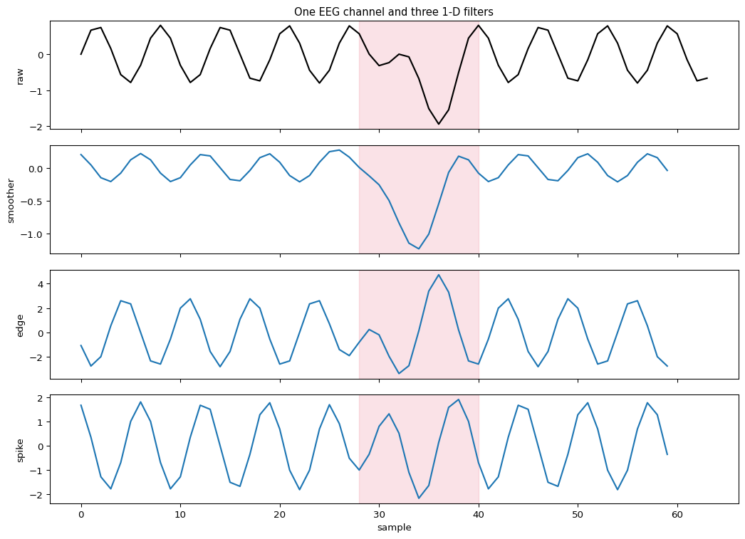
8. A 1-D Convolution on EEG
Everything above generalises down a dimension, which is the form used for signals. A 1-D kernel of length $k$ slides along time, and each filter learns a temporal motif — a sharp transient, a rhythm, a particular slope.
This is the layer that appears at the bottom of most EEG models, including the ones fed into the BERT-on-EEG walkthrough.
EEG: 64 samples at 64 Hz, with a burst at samples 28-40

          kernel                              values      sum                 detects
--------------------------------------------------------------------------------------
        smoother               [0.2 0.2 0.2 0.2 0.2]     1.00              slow trend
    edge / slope               [-1. -1.  0.  1.  1.]     0.00            rapid change
           spike          [-0.5 -1.   3.  -1.  -0.5]     0.00         sharp transient
--------------------------------------------------------------------------------------

position 30 of the spike detector, by hand:
   window  = [-0.3169 -0.2341 -0.     -0.0743 -0.6761]
   kernel  = [-0.5 -1.   3.  -1.  -0.5]
   (-0.3169)*(-0.5000) + (-0.2341)*(-1.0000) + (-0.0000)*(+3.0000) + (-0.0743)*(-1.0000) +
      (-0.6761)*(-0.5000)
   = +0.804886
   from the array: +0.804886   MATCH: True

1-D convolution MATCH with torch: True

The spike filter is near zero through the alpha rhythm and jumps during
the burst. In a trained network these five numbers would not be chosen -
they would be learned, by exactly the gradient descent shown in section 6.
9. Summary
| Concept | Formula / rule |
|---|---|
| Convolution | $O[i,j] = \sum_{u,v} I[i+u,j+v]K[u,v]$ |
| Output size | $\lfloor (\text{in} + 2p - k)/s \rfloor + 1$ |
| "Same" padding | $p = (k-1)/2$ |
| Filter weights | $(C_{out}, C_{in}, k, k)$ — independent of input size |
| Parameters | $C_{out}\cdot C_{in}\cdot k^2 + C_{out}$ |
| Pooling | max or mean over a window; no parameters |
| Kernel gradient | $\partial\mathcal{L}/\partial K[u,v] = \sum_{i,j}\partial\mathcal{L}/\partial O[i,j]\cdot I[i+u,j+v]$ |
| Library convention | Conv2d is cross-correlation — no kernel flip |
The one idea: reuse a small set of weights at every position. That single decision buys three things at once — a parameter count that does not grow with input size, a detector that works anywhere in the input, and a strong prior that what matters is local.
The prior is also the limitation. A convolution assumes nearby values are related and that the same pattern is meaningful everywhere. For images and signals that is true and enormously helpful. For tabular data where column order is arbitrary it is false, which is why convolutions are not used there and gradient-boosted trees are.
What is deliberately left out: dilated and transposed convolutions, 1×1 convolutions as channel mixing, depthwise-separable convolutions, batch normalisation, residual connections, and the architectures themselves (LeNet, ResNet, U-Net).