🌳 Decision Tree
A decision tree asks a sequence of yes/no questions about the features until it is confident enough to answer. The whole algorithm is one idea applied over and over:
Of every question I could ask, which one separates the classes best? Ask it, split the data in two, then repeat on each half.
Everything below is that loop, with the arithmetic written out. The data is a deliberately tiny EEG-flavoured table — 12 recordings — so every candidate split can be scored on the page, not just the winner.
The chain is:
impurity of a node → score every candidate split → take the best → recurse → leaves → prediction
At the end the hand-built tree is compared against scikit-learn's, node for node.
Display helpers ready: banner, step, check, expand, show_matrix, show_matmul, show_elementwise.
Tree diagram helper ready: draw_tree(root, title).
1. The Data
12 EEG recordings, three continuous features, and a binary label: did a seizure follow?
The table is small on purpose. A real tree searches thousands of thresholds; this one searches 33, and all 33 are printed later.
12 recordings x 3 features

    id      region   line_length    spike_rate           age   y_class    y_reg
-------------------------------------------------------------------------------
 rec00     frontal          12.0           0.5          24.0         0      0.2
 rec01    temporal          15.0           1.2          31.0         0      0.5
 rec02    temporal          42.0           6.8          58.0         1      6.4
 rec03   occipital          38.0           5.1          47.0         1      4.8
 rec04     frontal          11.0           0.3          19.0         0      0.1
 rec05    temporal          55.0           8.2          63.0         1      9.1
 rec06   occipital          40.0           1.9          35.0         1      3.5
 rec07    temporal          47.0           7.4          52.0         1      7.2
 rec08     frontal          14.0           0.8          28.0         0      0.3
 rec09   occipital          51.0           6.1          60.0         1      6.9
 rec10     frontal          45.0           2.4          41.0         0      1.6
 rec11    temporal          35.0           4.7          30.0         1      4.1
-------------------------------------------------------------------------------

class balance: 5 negative, 7 positive
y_reg mean = 3.7250, std = 3.0518
2. Gini Impurity
A node is pure when every sample in it has the same label. Gini impurity measures how far from pure a node is:
$$G = 1 - \sum_{k} p_k^2$$
where $p_k$ is the fraction of samples in the node belonging to class $k$.
Read it as a probability: $G$ is the chance that two samples drawn at random from the node (with replacement) have different labels.
- all one class → $p = 1$ → $G = 1 - 1 = 0$ (pure)
- 50/50 split → $G = 1 - 0.5^2 - 0.5^2 = 0.5$ (worst possible for 2 classes)
ROOT NODE - all 12 recordings

   class 0 (no seizure): 5 samples   ->  p_0 = 5/12 = 0.416667
   class 1 (seizure)   : 7 samples   ->  p_1 = 7/12 = 0.583333

   G = 1 - p_0^2 - p_1^2
     = 1 - (0.416667)^2 - (0.583333)^2
     = 1 - 0.173611 - 0.340278
     = 0.486111

Root impurity G_root = 0.486111
(0 would be pure, 0.5 is the worst case for two classes - this node is
 close to the worst case, which is why there is a lot to gain by splitting.)
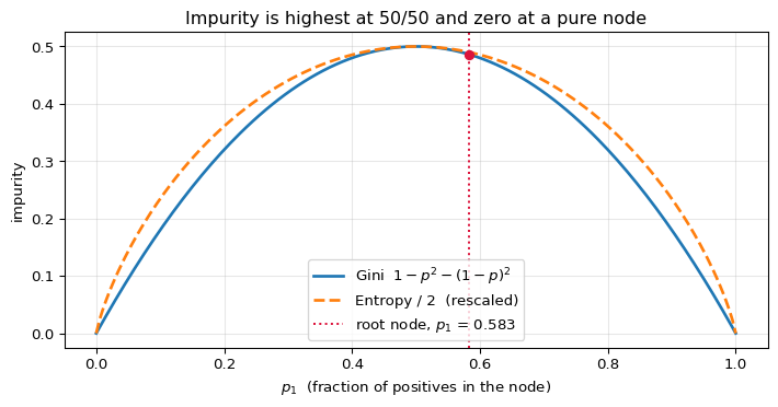
What impurity looks like
For two classes, Gini depends only on $p_1$. It is zero at both ends and peaks in the middle — a node that is 50/50 is maximally uninformative.
Both curves have the same shape and the same zeros, which is why swapping
Gini for entropy usually changes very little. Gini avoids the logarithm,
so it is the cheaper default.
3. Scoring One Candidate Split
A split is a feature and a threshold: is spike_rate $\le 3.55$? It sends every
sample either left or right. The quality of the split is how much impurity it removes:
$$G_{\text{children}} = \frac{n_L}{n}G_L + \frac{n_R}{n}G_R \qquad\qquad \text{Gain} = G_{\text{parent}} - G_{\text{children}}$$
The children are weighted by size, not counted equally — a pure child holding one sample is worth far less than a pure child holding six.
Candidate thresholds are the midpoints between consecutive distinct values of a feature. Anything between two observed values separates the data identically, so the midpoint is the natural representative.
CANDIDATE SPLIT:  spike_rate <= 3.55

    id    spike_rate    goes    y
----------------------------------
 rec00           0.5    LEFT    0
 rec01           1.2    LEFT    0
 rec02           6.8   RIGHT    1
 rec03           5.1   RIGHT    1
 rec04           0.3    LEFT    0
 rec05           8.2   RIGHT    1
 rec06           1.9    LEFT    1
 rec07           7.4   RIGHT    1
 rec08           0.8    LEFT    0
 rec09           6.1   RIGHT    1
 rec10           2.4    LEFT    0
 rec11           4.7   RIGHT    1
----------------------------------

LEFT  (6 samples): labels [0 0 0 1 0 0]
   p_0 = 5/6 = 0.833333,  p_1 = 1/6 = 0.166667
   G_L = 1 - 0.833333^2 - 0.166667^2 = 0.277778

RIGHT (6 samples): labels [1 1 1 1 1 1]
   p_0 = 0/6 = 0.000000,  p_1 = 6/6 = 1.000000
   G_R = 1 - 0.000000^2 - 1.000000^2 = 0.000000   <- PURE

weighted child impurity:
   (6/12) * 0.277778  +  (6/12) * 0.000000
   = 0.500000 * 0.277778  +  0.500000 * 0.000000
   = 0.138889 + 0.000000 = 0.138889

GAIN = G_root - weighted = 0.486111 - 0.138889 = 0.347222
4. Searching Every Candidate Split
The tree is greedy: it does not plan ahead, it simply scores every (feature, threshold) pair and takes the single best one.
With 3 features and 12 distinct values each there are $3 \times 11 = 33$ candidates. All of them are scored below, ranked by gain.
All 33 candidate splits, ranked by gain

rank       feature       thr   nL      G_L   nR      G_R   weighted      GAIN
-----------------------------------------------------------------------------
   1    spike_rate      3.55    6   0.2778    6   0.0000     0.1389    0.3472  <== BEST
   2   line_length     25.00    4   0.0000    8   0.2188     0.1458    0.3403
   3    spike_rate      1.55    4   0.0000    8   0.2188     0.1458    0.3403
   4    spike_rate      4.90    7   0.4082    5   0.0000     0.2381    0.2480
   5           age     44.00    7   0.4082    5   0.0000     0.2381    0.2480
   6   line_length     14.50    3   0.0000    9   0.3457     0.2593    0.2269
   7    spike_rate      1.00    3   0.0000    9   0.3457     0.2593    0.2269
   8           age     29.00    3   0.0000    9   0.3457     0.2593    0.2269
   9   line_length     36.50    5   0.3200    7   0.2449     0.2762    0.2099
  10    spike_rate      2.15    5   0.3200    7   0.2449     0.2762    0.2099
  11           age     33.00    5   0.3200    7   0.2449     0.2762    0.2099
  12    spike_rate      5.60    8   0.4688    4   0.0000     0.3125    0.1736
  13           age     49.50    8   0.4688    4   0.0000     0.3125    0.1736
  14   line_length     13.00    2   0.0000   10   0.4200     0.3500    0.1361
  15    spike_rate      0.65    2   0.0000   10   0.4200     0.3500    0.1361
  16           age     26.00    2   0.0000   10   0.4200     0.3500    0.1361
  17   line_length     39.00    6   0.4444    6   0.2778     0.3611    0.1250
  18           age     38.00    6   0.4444    6   0.2778     0.3611    0.1250
  19   line_length     46.00    9   0.4938    3   0.0000     0.3704    0.1157
  20    spike_rate      6.45    9   0.4938    3   0.0000     0.3704    0.1157
  21           age     55.00    9   0.4938    3   0.0000     0.3704    0.1157
  22           age     30.50    4   0.3750    8   0.3750     0.3750    0.1111
  23   line_length     49.00   10   0.5000    2   0.0000     0.4167    0.0694
  24    spike_rate      7.10   10   0.5000    2   0.0000     0.4167    0.0694
  25           age     59.00   10   0.5000    2   0.0000     0.4167    0.0694
  26   line_length     41.00    7   0.4898    5   0.3200     0.4190    0.0671
  27   line_length     11.50    1   0.0000   11   0.4628     0.4242    0.0619
  28    spike_rate      0.40    1   0.0000   11   0.4628     0.4242    0.0619
  29           age     21.50    1   0.0000   11   0.4628     0.4242    0.0619
  30   line_length     53.00   11   0.4959    1   0.0000     0.4545    0.0316
  31    spike_rate      7.80   11   0.4959    1   0.0000     0.4545    0.0316
  32           age     61.50   11   0.4959    1   0.0000     0.4545    0.0316
  33   line_length     43.50    8   0.5000    4   0.3750     0.4583    0.0278
-----------------------------------------------------------------------------

WINNER: spike_rate <= 3.55   (gain 0.347222)

runner-up: line_length <= 25.00  (gain 0.340278)
The winner beats it outright, so the root question is unambiguous here.
Deeper in the tree that stops being true - see section 7.
Why the winner wins
spike_rate <= 3.55 sends all six high-spike-rate recordings into a node that is
perfectly pure ($G_R = 0$): every one of them had a seizure. That single question
removes most of the uncertainty in the dataset, which is exactly what the gain measures.
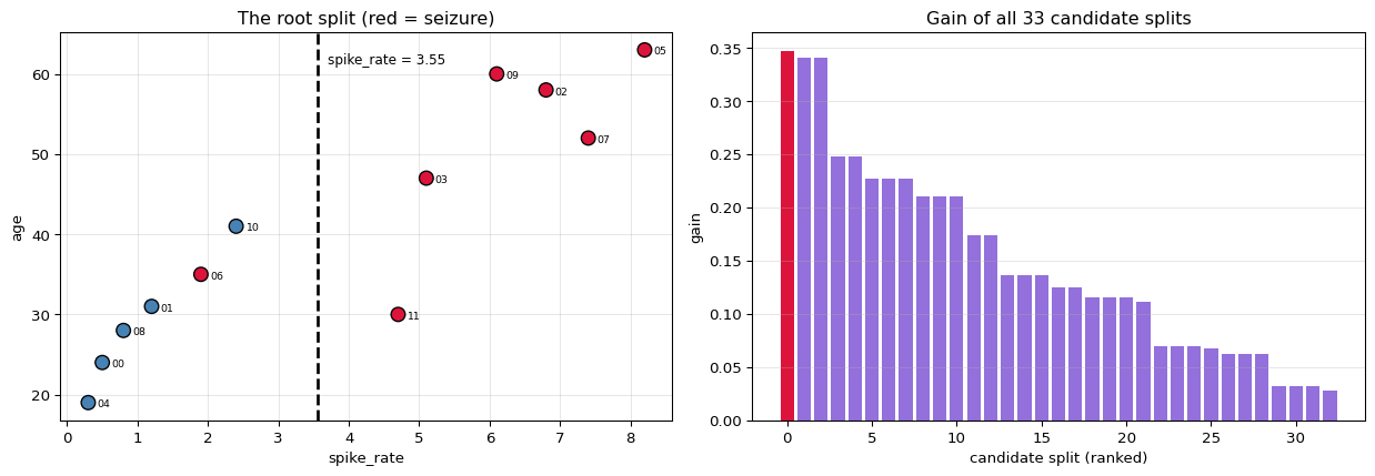
Left: one vertical line separates every high-spike-rate recording, all of
which are seizures. Right: that split's gain stands clearly above the rest.
How a split is actually found, feature by feature
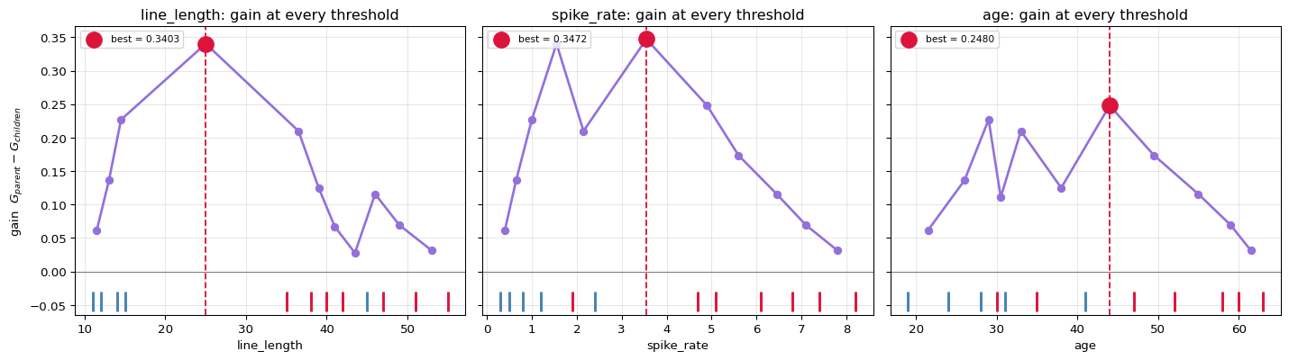
The search is mechanical. For each feature: sort the values, walk across every midpoint, and evaluate the gain there. The plots below show that walk directly — one line per feature, one point per candidate threshold.
Reading them: the dots along the bottom are the 12 recordings placed at their feature value (red = seizure). The curve above is the gain the tree would earn by cutting at that point. The peak of the curve is the split that feature would contribute, and the tree simply takes the highest peak across all three.
best threshold per feature (the peak of each curve):

     feature   best threshold       gain
----------------------------------------
  spike_rate             3.55     0.3472  <== the tree picks this
 line_length            25.00     0.3403
         age            44.00     0.2480
----------------------------------------

Notice the shape: gain rises as the cut approaches the boundary between
classes and falls away on either side. A feature that separated the classes
perfectly would peak at the root impurity itself (0.4861 here).
The root split as a diagram
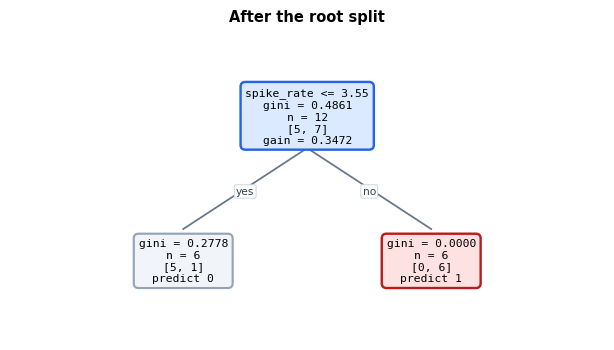
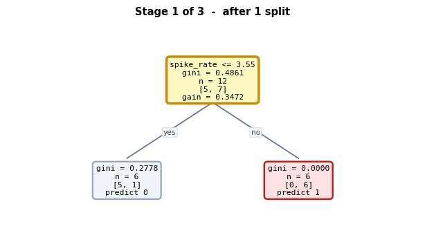
The same result drawn as a tree. Every number inside a node is one of the quantities
computed above: the question being asked, the node's Gini impurity, how many recordings
reach it, the class counts [negatives, positives], and the gain the split earned.
LEFT  (6 rows): gini 0.2778 - still mixed, so it will be split again
RIGHT (6 rows): gini 0.0000 - PURE, so it becomes a leaf and stops
5. Recursion — Growing the Whole Tree
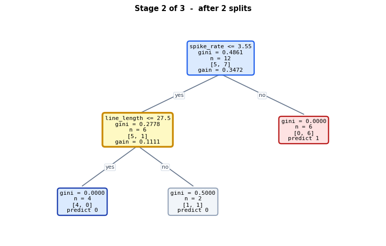
The right child is already pure, so it becomes a leaf. The left child still mixes five negatives with one positive, so the identical search runs again — but now only on those six rows.
This is the entire algorithm: the same function, called on smaller and smaller subsets, stopping when a node is pure or a limit is reached.
Growing the tree, one recursive call per node:

NODE depth=0  n=12  [5 neg, 7 pos]  G=0.4861
   -> best split: spike_rate <= 3.55  (gain 0.3472)  sends 6 left, 6 right
   NODE depth=1  n=6  [5 neg, 1 pos]  G=0.2778
      -> best split: line_length <= 27.5  (gain 0.1111)  sends 4 left, 2 right
      NODE depth=2  n=4  [4 neg, 0 pos]  G=0.0000
         -> PURE, becomes a LEAF predicting class 0
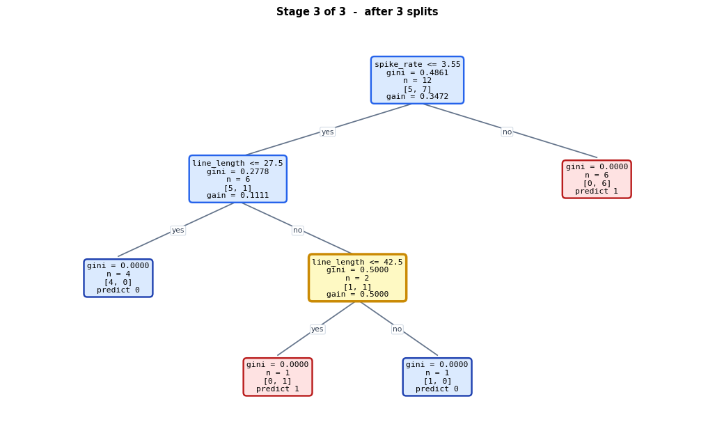
      NODE depth=2  n=2  [1 neg, 1 pos]  G=0.5000
         -> best split: line_length <= 42.5  (gain 0.5000)  sends 1 left, 1 right
         NODE depth=3  n=1  [0 neg, 1 pos]  G=0.0000
            -> PURE, becomes a LEAF predicting class 1
         NODE depth=3  n=1  [1 neg, 0 pos]  G=0.0000
            -> PURE, becomes a LEAF predicting class 0
   NODE depth=1  n=6  [0 neg, 6 pos]  G=0.0000
      -> PURE, becomes a LEAF predicting class 1
Watching the tree grow, one split at a time
The same recursion drawn stage by stage. At each stage the node about to be split is outlined in yellow, grey nodes are still impure and waiting their turn, and coloured nodes are finished leaves.
Every box carries the criteria used to make the decision: the question, the Gini impurity, the number of recordings, the class counts, and the gain earned.
the finished tree uses 3 splits, so there are 3 growth stages
The finished tree
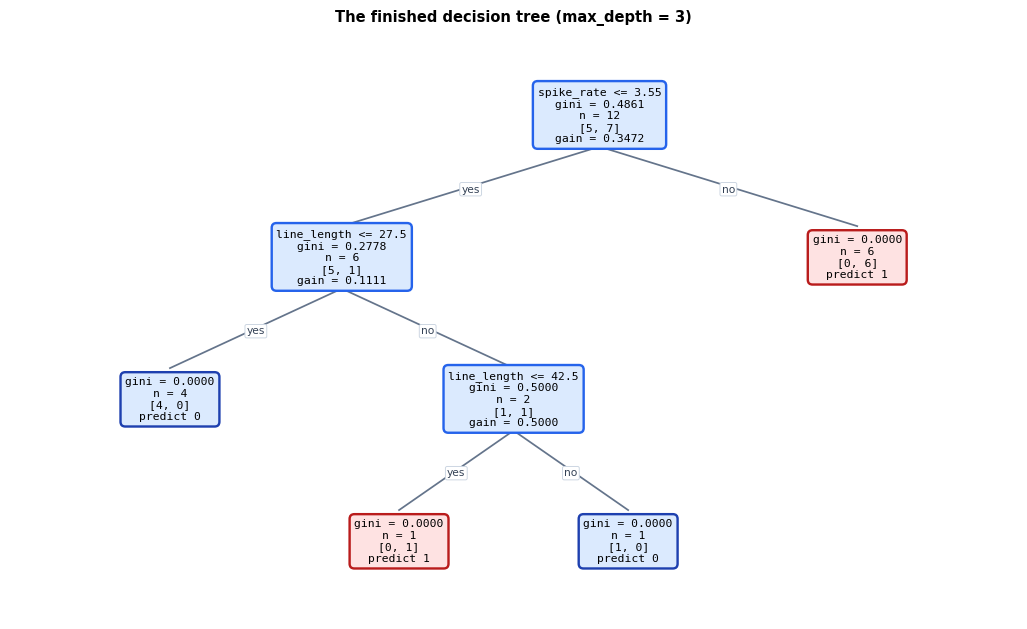
Four leaves, every one of them pure. Read a path by following the answers from the top.
Reading a leaf: [a, b] is [negatives, positives] reaching that leaf.
gini = 0 in every leaf means each one contains a single class.

The four decision rules this tree encodes:

   IF spike_rate <= 3.55 AND line_length <= 27.5
      -> predict 0   (n=4, [4, 0], gini=0.000)

   IF spike_rate <= 3.55 AND NOT(line_length <= 27.5) AND line_length <= 42.5
      -> predict 1   (n=1, [0, 1], gini=0.000)

   IF spike_rate <= 3.55 AND NOT(line_length <= 27.5) AND NOT(line_length <= 42.5)
      -> predict 0   (n=1, [1, 0], gini=0.000)

   IF NOT(spike_rate <= 3.55)
      -> predict 1   (n=6, [0, 6], gini=0.000)
[spike_rate <= 3.55] n=12  G=0.4861
|-- yes: [line_length <= 27.5] n=6  G=0.2778
    |-- yes: LEAF  predict 0   n=4  [4 neg, 0 pos]  G=0.000   ['rec00', 'rec01', 'rec04', 'rec08']
    |-- no : [line_length <= 42.5] n=2  G=0.5000
        |-- yes: LEAF  predict 1   n=1  [0 neg, 1 pos]  G=0.000   ['rec06']
        |-- no : LEAF  predict 0   n=1  [1 neg, 0 pos]  G=0.000   ['rec10']
|-- no : LEAF  predict 1   n=6  [0 neg, 6 pos]  G=0.000   ['rec02', 'rec03', 'rec05', 'rec07', 'rec09', 'rec11']

depth = 3, leaves = 4

Every leaf is pure, so this tree classifies all 12 training recordings
correctly. On 12 samples that is not evidence of a good model - it is
exactly the overfitting a single deep tree is prone to.
6. Prediction — Walking a Sample Down
Prediction costs almost nothing: compare, branch, repeat. A tree of depth $d$ needs at most $d$ comparisons regardless of how much data it was trained on.
rec06: line_length=40, spike_rate=1.9, age=35   (true label 1)
   is spike_rate (1.9) <= 3.55?  YES -> left
   is line_length (40) <= 27.5?  NO  -> right
   is line_length (40) <= 42.5?  YES -> left
   reached a leaf -> predict class 1
   predicted 1   correct: True

rec10: line_length=45, spike_rate=2.4, age=41   (true label 0)
   is spike_rate (2.4) <= 3.55?  YES -> left
   is line_length (45) <= 27.5?  NO  -> right
   is line_length (45) <= 42.5?  NO  -> right
   reached a leaf -> predict class 0
   predicted 0   correct: True

rec05: line_length=55, spike_rate=8.2, age=63   (true label 1)
   is spike_rate (8.2) <= 3.55?  NO  -> right
   reached a leaf -> predict class 1
   predicted 1   correct: True

predictions : [0 0 1 1 0 1 1 1 0 1 0 1]
true labels : [0 0 1 1 0 1 1 1 0 1 0 1]
training accuracy: 1.0000
7. Checking Against scikit-learn
Everything above was computed from the formulas alone. Fitting
DecisionTreeClassifier(criterion="gini", max_depth=3) on the same table should
reproduce the same root question, the same impurities, and the same predictions.
Deeper in the tree it will not match node for node — the reason is a tie, and it is printed at the end of this section.
scikit-learn's tree:

|--- spike_rate <= 3.55
|   |--- age <= 33.00
|   |   |--- class: 0
|   |--- age >  33.00
|   |   |--- line_length <= 42.50
|   |   |   |--- class: 1
|   |   |--- line_length >  42.50
|   |   |   |--- class: 0
|--- spike_rate >  3.55
|   |--- class: 1

 node       feature       thr    n   impurity
----------------------------------------------
    0    spike_rate      3.55   12   0.486111
    1           age     33.00    6   0.277778
    2          LEAF              4   0.000000
    3   line_length     42.50    2   0.500000
    4          LEAF              1   0.000000
    5          LEAF              1   0.000000
    6          LEAF              6   0.000000
----------------------------------------------

root feature   : ours =   spike_rate | sklearn =   spike_rate  MATCH: True
root threshold : ours =       3.5500 | sklearn =       3.5500  MATCH: True
root impurity  : ours =     0.486111 | sklearn =     0.486111  MATCH: True
depth          : ours = 3, sklearn = 3  MATCH: True
leaf count     : ours = 4, sklearn = 4  MATCH: True
predictions    : MATCH: True


TIES - why the two trees are not identical deeper down

At the depth-1 left node, 3 different questions all reach the
same best gain of 0.111111:

       line_length <= 27.50    gain 0.111111  <- ours
        spike_rate <= 1.55     gain 0.111111
               age <= 33.00    gain 0.111111  <- sklearn

Our search breaks the tie by lowest feature index; sklearn breaks it its own
way. Both are valid greedy trees. What the data determines is the GAIN, not
which of the tied questions gets asked - and since the tied splits separate
these rows identically, the predictions come out the same either way.
8. Gini vs Entropy
The other common impurity measure is entropy:
$$H = -\sum_k p_k \log_2 p_k \qquad\text{and}\qquad \text{Information Gain} = H_{\text{parent}} - \sum_{\text{child}} \frac{n_c}{n} H_c$$
Entropy is steeper near the middle, so it slightly prefers balanced splits. In practice the two almost always choose the same question — as they do here.
Root:   Gini = 0.486111      Entropy = 0.979869 bits
        H = -(5/12)*log2(5/12) - (7/12)*log2(7/12)
          = -0.4167*(-1.2630) - 0.5833*(-0.7776)
          = 0.979869

     feature       thr   gini gain   info gain
----------------------------------------------
  spike_rate      3.55      0.3472      0.6549
 line_length     25.00      0.3403      0.6175
  spike_rate      1.55      0.3403      0.6175
  spike_rate      4.90      0.2480      0.4764
         age     44.00      0.2480      0.4764
 line_length     14.50      0.2269      0.4067
----------------------------------------------

best by Gini    : spike_rate <= 3.55
best by Entropy : spike_rate <= 3.55
same question?  : True

sklearn with criterion='entropy' picks: spike_rate <= 3.55
9. Where Trees Break
Three properties follow directly from the arithmetic above, and each one motivates a model later in this series.
Greedy, never revisited. The root is chosen to be locally best and is never reconsidered. A pair of questions that is jointly excellent but individually mediocre will never be found.
Axis-aligned only. Every question has the form feature $\le$ threshold, so every boundary is a vertical or horizontal cut. A diagonal boundary has to be approximated with a staircase.
High variance. Every leaf here is pure — the tree memorised 12 recordings. Change one label and the structure can change completely, as shown below.
That last property is the opening for the next notebook: if a single deep tree is unstable, average many of them. That is a random forest.
Sensitivity: flip ONE label and refit

original root question: spike_rate <= 3.55

 flipped               new root question   changed?
----------------------------------------------------
   rec00              spike_rate <= 3.55         no
   rec01             line_length <= 14.5        YES
   rec02             line_length <= 25.0        YES
   rec03             line_length <= 25.0        YES
   rec04              spike_rate <= 3.55         no
   rec05             line_length <= 25.0        YES
   rec06              spike_rate <= 3.55         no
   rec07             line_length <= 25.0        YES
   rec08              spike_rate <= 3.55         no
   rec09             line_length <= 25.0        YES
   rec10             line_length <= 25.0        YES
   rec11             line_length <= 36.5        YES
----------------------------------------------------

8 of 12 single-label flips change the very first question.
A model this sensitive to one sample has high variance - averaging many such
trees is exactly what bagging and random forests do.
10. Summary
| Stage | Formula | Result here |
|---|---|---|
| Node impurity | $G = 1 - \sum_k p_k^2$ | root $G = 0.4861$ |
| Split quality | $\frac{n_L}{n}G_L + \frac{n_R}{n}G_R$ | best $= 0.1389$ |
| Gain | $G_{\text{parent}} - G_{\text{children}}$ | $0.3472$ |
| Candidates searched | midpoints of distinct values | 33 |
| Winning question | — | spike_rate <= 3.55 |
| Final tree | greedy recursion | depth 3, 4 pure leaves |
| Prediction cost | $\le$ depth comparisons | 3 |
What is deliberately left out: pruning (cost-complexity $\alpha$), missing-value
surrogate splits, multi-class targets beyond two, regression trees (variance instead of
Gini), and any form of regularisation other than max_depth.
What carries forward: every model in the rest of this series is built out of this same greedy split search. Random forests average many of these trees; gradient boosting machines fit them one after another to each other's errors.
References
- Classification and Regression Trees