🗜 DeepSeek-V4: Compressed Sparse Attention and Muon
DeepSeek-V4 from Scratch in NumPy — Compressed Sparse Attention, Manifold-Constrained Residuals, Muon
This notebook works through the architecture of DeepSeek-V4 (DeepSeek-AI, technical report arXiv:2606.19348) in pure NumPy, on an eight-token sentence, with every intermediate number printed.
DeepSeek-V4 is a Mixture-of-Experts model built for one-million-token context. Two variants: V4-Flash (284B total, 13B activated) and V4-Pro (1.6T total, 49B activated). The headline claim is efficiency — in the 1M-token setting the KV cache is about 2% the size of a BF16 GQA-8 baseline, and a single token's inference costs 27% of the FLOPs of DeepSeek-V3.2 with 10% of the KV cache.
Three ideas do that work, and this notebook takes each one apart:
| § | Mechanism | Equations | The problem it solves |
|---|---|---|---|
| 2 | mHC — Manifold-Constrained Hyper-Connections | 1–8 | Widening the residual stream makes deep stacks numerically unstable |
| 3 | CSA — Compressed Sparse Attention | 9–19 | KV cache and attention FLOPs at long context |
| 4 | HCA — Heavily Compressed Attention | 20–26 | The same, more aggressively, on alternating layers |
| 5 | Normalisation, partial RoPE, sliding window, attention sink | 27 | The details that make the above actually train |
| 6 | DeepSeekMoE, with the V4 changes | — | Sparsity, and what changed from V3 |
| 7 | Muon with hybrid Newton–Schulz | 28 | Faster, more stable optimisation than AdamW |
Everything is computed on a deliberately tiny model so the matrices fit on a screen. The real configuration is quoted alongside each one so you can see which numbers are toy and which are DeepSeek's.
No code is shown on this page — only the explanations, the formulas, and the numbers that come out.
1. The problem, in numbers
Attention cost is the reason this architecture looks the way it does. Before any mechanism, it is worth seeing the size of the thing being fixed.
A standard GQA-8 layer with head dimension 128 stores, for every token, 8 key vectors and 8 value vectors. In BF16 that is
$$\text{bytes per token per layer} = 2 \times n_{\text{kv}} \times d_{\text{head}} \times 2 = 2 \times 8 \times 128 \times 2 = 4096\ \text{bytes}$$
Multiply by a million tokens and by the number of layers and the number stops being reasonable. That is the wall DeepSeek-V4 is built against.
Display helpers ready: banner, step, check, expand, show_matrix, show_matmul, show_elementwise.
==============================================================================
  THE LONG-CONTEXT KV CACHE PROBLEM
==============================================================================
  baseline: BF16 GQA-8, head dim 128
    per token per layer = 2 x 8 x 128 x 2 B = 4,096 B
    x 1,000,000 tokens x 43 layers = 164 GiB

  164 GiB is the cache for ONE request at 1M context.
  An 80 GiB accelerator holds none of it, let alone a batch of them.

Where DeepSeek-V4 spends its cache instead
==============================================================================
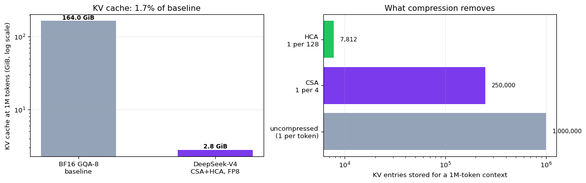
  CSA compresses every m=4 tokens into one KV entry   -> 1,000,000 -> 250,000 entries
  HCA compresses every m'=128 tokens into one entry -> 1,000,000 -> 7,812 entries

  and the entries are shared across all heads (MQA), not one per head:
    CSA: 250,000 x 512 values
    HCA: 7,812 x 512 values

  The paper reports the combined effect as ~2% of the BF16 GQA-8
  baseline at 1M context. Section 8 rebuilds that number.

The other half of the problem: attention FLOPs
==============================================================================
  Even with a short cache, dense attention still scores every entry.
  CSA scores 250,000 compressed entries with a cheap indexer, then
  runs full attention over only the top-k = 512 of them.

    dense over compressed : 250,000 entries attended
    CSA sparse            : 512 entries attended   (0.2% of them)
2. Manifold-Constrained Hyper-Connections (mHC)
2.1 What a hyper-connection is
An ordinary transformer block is
$$x_{l+1} = x_l + \mathcal{F}_l(x_l)$$
one residual stream of width $d$. Hyper-connections (Zhu et al., 2025) widen that stream by a factor $n_{\text{hc}}$, so the state carried between blocks is a matrix $X_l \in \mathbb{R}^{n_{\text{hc}} \times d}$ rather than a vector. Three small learned maps connect it to the block:
- $A_l \in \mathbb{R}^{1 \times n_{\text{hc}}}$ — mixes the streams down to the one vector the layer actually sees
- $B_l \in \mathbb{R}^{n_{\text{hc}} \times n_{\text{hc}}}$ — mixes the streams among themselves
- $C_l \in \mathbb{R}^{n_{\text{hc}} \times 1}$ — writes the layer output back out across the streams
$$X_{l+1} = B_l X_l + C_l\,\mathcal{F}_l(A_l X_l) \qquad (1)$$
The layer $\mathcal{F}_l$ still takes and returns a $d$-vector, so nothing inside the block changes — the width $n_{\text{hc}}$ is a new scaling axis that costs almost nothing, since $n_{\text{hc}} \ll d$. DeepSeek-V4 uses $n_{\text{hc}} = 4$; this notebook uses 3 so the matrices print small.
Setting $n_{\text{hc}} = 1$, $A = B = C = 1$ recovers the ordinary residual connection exactly — worth checking, and the notebook does.
==============================================================================
  HYPER-CONNECTIONS: THE RESIDUAL STREAM BECOMES A MATRIX
==============================================================================

Eq 1  X_{l+1} = B_l X_l + C_l F_l(A_l X_l)
==============================================================================
  n_hc = 3  ->  the state between blocks is (3 x 8), not (8,)

  shapes:
    X_l      (3 x 8)     the widened residual state
    A_l      (1 x 3)     stream mixer, down to what the layer sees
    A_l X_l  (1 x 8)     <- the layer input: still just d-dimensional
    B_l      (3 x 3)     stream-to-stream mixing
    C_l      (3 x 1)     writes the layer output back to the streams

Sanity: n_hc = 1 with A = B = C = 1 must be the ordinary residual
==============================================================================
  hyper-connection : [0.0272 0.4043 0.1843 1.0573 0.0078] ...
  x + F(x)         : [0.0272 0.4043 0.1843 1.0573 0.0078] ...
  max|diff| = 0.00e+00   MATCH: True

  So hyper-connections strictly generalise the residual connection.
2.2 Why $B_l$ must be constrained
Equation (1) applies $B_l$ to the residual state at every layer. Across $L$ layers the stream has been multiplied by $B_L B_{L-1} \cdots B_1$. If those matrices have spectral norm above 1, the product grows geometrically — with 43 layers, a spectral norm of 1.1 is a factor of $1.1^{43} \approx 60$, and 1.3 is a factor of over 40,000. That is the numerical instability the paper reports when scaling plain hyper-connections.
mHC's fix is to constrain $B_l$ to the Birkhoff polytope — the set of doubly stochastic matrices:
$$B_l \in \mathcal{M} := \{M \in \mathbb{R}^{n\times n} \mid M\mathbf{1}_n = \mathbf{1}_n,\ \mathbf{1}_n^T M = \mathbf{1}_n^T,\ M \geqslant 0\} \qquad (2)$$
Non-negative, every row sums to 1, every column sums to 1. Two properties follow, and both matter:
- $\|B_l\|_2 \leqslant 1$ — the map is non-expansive, so signals cannot blow up going forward or backward.
- $\mathcal{M}$ is closed under multiplication — a product of doubly stochastic matrices is doubly stochastic, so the guarantee survives stacking to any depth.
The demonstration below is the whole argument for mHC in one table.
==============================================================================
  WHY THE RESIDUAL MIXER MUST BE NON-EXPANSIVE
==============================================================================

A spectral norm slightly above 1, compounded over 43 layers
==============================================================================
    ||B||_2        ||B||^43   effect on the residual stream
  --------------------------------------------------------------
       0.90         0.01078   shrinks to nothing
       1.00               1   stable
       1.05            8.15   grows
       1.10           60.24   grows
       1.30       7.935e+04   explodes
  --------------------------------------------------------------
  Doubly stochastic guarantees the 1.00 row, for every layer, forever.

Property 1: doubly stochastic => spectral norm exactly bounded by 1
==============================================================================
    seed 0:  ||B||_2 = 1.000000   row sums [1. 1. 1.]   col sums [1. 1. 1.]
    seed 1:  ||B||_2 = 1.000000   row sums [1. 1. 1.]   col sums [1. 1. 1.]
    seed 2:  ||B||_2 = 1.000000   row sums [1. 1. 1.]   col sums [1. 1. 1.]
    seed 3:  ||B||_2 = 1.000000   row sums [1. 1. 1.]   col sums [1. 1. 1.]

  The top singular value is 1.000000 every time - exactly, not
  approximately, and the reason is a theorem rather than an accident:
    Birkhoff-von Neumann says every doubly stochastic matrix is a
    convex combination of permutation matrices. Each permutation has
    spectral norm 1, and the spectral norm is convex, so ||B||_2 <= 1.
    And B1 = 1 forces ||B||_2 >= 1. Hence exactly 1.

Property 2: closed under multiplication (so depth is safe)
==============================================================================
   layers   ||prod||_2   max row sum   max col sum
  ------------------------------------------------
        1     1.000000      1.000000      1.000000
        2     1.000000      1.000000      1.000000
        5     1.000000      1.000000      1.000000
       10     1.000000      1.000000      1.000000
       20     1.000000      1.000000      1.000000
       43     1.000000      1.000000      1.000000
  ------------------------------------------------
  43 layers deep and the product is still doubly stochastic,
  still non-expansive. Compare the 1.1 row of the first table.

The contrast: unconstrained B, the same 43 layers
==============================================================================
    after  1 layers: ||prod||_2 = 1.9959e+00
    after  5 layers: ||prod||_2 = 3.0658e+00
    after 10 layers: ||prod||_2 = 5.1688e-01
    after 20 layers: ||prod||_2 = 2.3549e-01
    after 43 layers: ||prod||_2 = 1.7051e-04

  This is why plain hyper-connections were reported as unstable.
2.3 Where $A_l$, $B_l$, $C_l$ come from
They are not free parameters. Each is generated from the input itself — a dynamic, input-dependent part plus a static learned bias. First the widened state is flattened and normalised:
$$\hat{X}_l = \operatorname{RMSNorm}(\operatorname{vec}(X_l)) \in \mathbb{R}^{1 \times n_{\text{hc}}d}$$
then
$$\tilde{A}_l = \alpha_l^{\mathrm{pre}} \cdot (\hat{X}_l W_l^{\mathrm{pre}}) + S_l^{\mathrm{pre}} \qquad (3)$$ $$\tilde{B}_l = \alpha_l^{\mathrm{res}} \cdot \operatorname{Mat}(\hat{X}_l W_l^{\mathrm{res}}) + S_l^{\mathrm{res}} \qquad (4)$$ $$\tilde{C}_l = \alpha_l^{\mathrm{post}} \cdot (\hat{X}_l W_l^{\mathrm{post}})^T + S_l^{\mathrm{post}} \qquad (5)$$
$\operatorname{Mat}(\cdot)$ reshapes a $1 \times n_{\text{hc}}^2$ vector into an $n_{\text{hc}} \times n_{\text{hc}}$ matrix. The gates $\alpha^{\mathrm{pre}}, \alpha^{\mathrm{res}}, \alpha^{\mathrm{post}}$ are learnable scalars initialised to small values — so at the start of training the maps are essentially the static biases, and the dynamic part fades in.
Then the constraints. $A_l$ and $C_l$ are squashed to be non-negative and bounded, which prevents the streams from cancelling each other:
$$A_l = \sigma(\tilde{A}_l) \qquad (6) \qquad\qquad C_l = 2\,\sigma(\tilde{C}_l) \qquad (7)$$
Note the factor 2 on $C_l$: $\sigma$ alone caps the output-write at 1, and the paper allows the layer output to be written with weight up to 2.
==============================================================================
  mHC PARAMETERISATION (EQ 3-7), BY HAND
==============================================================================

Flatten and RMSNorm the state  (the input to all three generators)
==============================================================================
  vec(X_l) shape (1, 24)   (n_hc x d = 3 x 8 = 24)
  mean square = 0.314985   rms = 0.561236
  Xhat[:8] = [ 1.8073 -0.4981  0.0351  0.4357 -0.8434  0.0022 -0.001  -1.8759]

Eq 3-5: dynamic component + static bias
==============================================================================
  alpha_pre = alpha_res = alpha_post = 0.05  (small at init)

  A~ (1 x 3)  = [-0.8969 -0.5156 -0.0245]
  B~ (3 x 3) =
        [-0.0405  0.1218 -0.0654]
        [ 0.0326  0.2282 -0.2934]
        [-0.1119 -0.5032  0.283 ]
  C~ (3 x 1)  = [0.0637 0.1459 0.4918]

Eq 6-7: squash A and C so the streams cannot cancel
==============================================================================
  A = sigma(A~)     = [0.2897 0.3739 0.4939]     all in (0, 1)   -> True
  C = 2 sigma(C~)   = [1.0318 1.0728 1.2411]     all in (0, 2)   -> True

  Non-negative means every stream contributes with the same sign.
  Nothing can be subtracted away, which is the 'signal cancellation'
  the paper is guarding against.
2.4 Projecting $B_l$ onto the Birkhoff polytope: Sinkhorn–Knopp
$\tilde{B}_l$ from equation (4) is an arbitrary matrix. It has to become doubly stochastic. The projection is Sinkhorn–Knopp: exponentiate to force positivity, then alternately normalise columns and rows until both sum to 1.
$$M^{(0)} = \exp(\tilde{B}_l), \qquad M^{(t)} = \mathcal{T}_r\big(\mathcal{T}_c(M^{(t-1)})\big) \qquad (8)$$
with $B_l = M^{(t_{\max})}$ and DeepSeek using $t_{\max} = 20$.
Each half-step is trivial — divide every column by its sum, then every row by its sum. The subtlety is that fixing the rows breaks the columns again, slightly. The iteration works because it breaks them less each time; it converges geometrically. Watch the two error columns below fall together.
==============================================================================
  SINKHORN-KNOPP: PROJECTING B~ ONTO THE DOUBLY STOCHASTIC MANIFOLD
==============================================================================

Eq 8, iterated by hand
==============================================================================
  M(0) = exp(B~)  -- positive, but sums are arbitrary:
        [0.9603 1.1295 0.9367]
        [1.0331 1.2563 0.7458]
        [0.8941 0.6046 1.3272]
    row sums [3.0266 3.0352 2.8259]   col sums [2.8875 2.9904 3.0097]

   iter   max|rowsum-1|   max|colsum-1|    ||M||_2
  --------------------------------------------------
      1        1.11e-16        9.09e-03   1.000027
      2        2.22e-16        4.36e-04   1.000000
      3        1.11e-16        2.09e-05   1.000000
      4        0.00e+00        9.99e-07   1.000000
      5        0.00e+00        4.78e-08   1.000000
     10        1.11e-16        1.20e-14   1.000000
     20        0.00e+00        0.00e+00   1.000000
  --------------------------------------------------

  B = M(20):
        [0.3256 0.3728 0.3016]
        [0.3485 0.4126 0.2389]
        [0.3259 0.2146 0.4595]
    row sums [1. 1. 1.]
    col sums [1. 1. 1.]
    all entries >= 0 : True
    singular values  : [1.     0.2187 0.0167]
    ||B||_2 = 1.00000000 <= 1 : True

Note which normalisation goes last, and why the row error is smaller
==============================================================================
  Eq 8 is T_r(T_c(.)) - columns first, then rows. So after the final
  half-step the ROWS are exactly 1 and the columns are 1 only to the
  accuracy reached so far. That asymmetry is visible in the table above:
    |rowsum-1| = 0.00e+00   <- exact, it was normalised last
    |colsum-1| = 0.00e+00   <- the residual error

  At t_max=20 the column error is far below bf16 resolution (~4e-3),
  so the matrix is doubly stochastic as far as the model can tell.
2.5 One full mHC block
All the pieces, applied through equation (1) once. The thing to watch in the output is the last table: the mHC block leaves the norm of the residual state essentially unchanged, while the unconstrained version does not.
==============================================================================
  ONE mHC BLOCK, END TO END (EQ 1)
==============================================================================

Eq 1: X_{l+1} = B X_l + C F(A X_l)
==============================================================================
  A X_l  ((1, 3) @ (3, 8) -> (1, 8))  = the d-vector the layer sees
    [ 0.6865  0.0904 -0.0533 -0.42    0.4654 -0.0125 -0.1693 -0.0297]

  F(A X_l) = [ 0.425   0.1392 -0.2735 -0.5753 -0.1163 -0.2123 -0.05   -0.3658]

  B X_l      ((3, 8))   stream mixing
  C F(A X_l) ((3, 8))   output written back, weighted per stream
    C = [1.0318 1.0728 1.2411]  -> stream 2 receives the most

Norm bookkeeping: what mHC buys
==============================================================================
                            ||X||_F     ratio
  --------------------------------------------
  before the block           2.7495    1.0000
  after B X (mixing)         1.4482    0.5267   <= 1, guaranteed
  after full block           2.9194    1.0618   grows only by what F added
  --------------------------------------------
  The mixing step can never amplify. Any growth in the residual stream
  comes from the layer's own output, which is what you want -- it is
  the uncontrolled compounding of B that mHC removes.

The same block with an UNCONSTRAINED B, for contrast
==============================================================================
  ||B_mHC||_2 = 1.0000      ||B_unc||_2 = 1.8651

   block     ||X|| mHC    ||X|| unconstrained
  --------------------------------------------
       1        2.9194             3.2679e+00
       5       15.0048             1.0621e+01
      10       34.7637             3.5633e+01
      15       55.1156             1.4019e+02
      20       75.5308             5.6424e+02
  --------------------------------------------
  Same layer, same C, same input. Only the constraint on B differs.
3. Compressed Sparse Attention (CSA)
CSA attacks the cache and the FLOPs in two separate stages:
- Compress — every $m$ tokens collapse into one KV entry, so the sequence the attention sees is $n/m$ long. DeepSeek uses $m=4$.
- Select — a cheap "lightning indexer" scores those compressed entries and full attention runs over only the top $k$. DeepSeek uses $k=512$.
Stage 1 shrinks the cache. Stage 2 shrinks the compute. They are independent, and the paper applies both.
3.1 Building the compressed KV entries
Two separate KV projections and two compression-weight projections are computed from the hidden states $H \in \mathbb{R}^{n \times d}$:
$$C^a = H W^{aKV}, \quad C^b = H W^{bKV} \qquad (9)$$ $$Z^a = H W^{aZ}, \quad Z^b = H W^{bZ} \qquad (10)$$
Then compressed entry $i$ pools $2m$ source tokens — $m$ from the $a$ stream at positions $[mi,\ m(i{+}1))$ and $m$ from the $b$ stream at the previous block $[m(i{-}1),\ mi)$ — with a softmax over all $2m$ of them, plus learnable positional biases $B^a, B^b \in \mathbb{R}^{m \times c}$:
$$[S^a; S^b] = \operatorname{Softmax}_{\text{row}}\big([Z^a + B^a;\ Z^b + B^b]\big) \qquad (11)$$ $$C^{\text{Comp}}_i = \sum_{j=mi}^{m(i+1)-1} S^a_j \odot C^a_j \;+\; \sum_{j=m(i-1)}^{mi-1} S^b_j \odot C^b_j \qquad (12)$$
Two things are easy to misread here:
- The softmax is per channel, not per token. Each of the $c$ dimensions gets its own distribution over the $2m$ contributing tokens. That is why $B^a$ is $m \times c$ and why $\odot$ appears rather than a scalar weight.
- Each entry draws on $2m$ tokens, but consecutive entries overlap — the $b$-half of entry $i$ covers the same positions as the $a$-half of entry $i-1$. So the compression ratio is $1/m$, not $1/2m$. The overlap exists so information near a block boundary is not cut in half.
At $i=0$ there is no previous block, so $Z^b$ is padded with $-\infty$ (weight zero after softmax) and $C^b$ with zeros.
==============================================================================
  CSA STAGE 1: COMPRESSING THE KV CACHE (EQ 9-12)
==============================================================================

Eq 9-10: two KV streams and two weight streams
==============================================================================
  H (8 x 8) -> Ca, Cb, Za, Zb each (8 x 4)
  m = 2, so 8 tokens -> 4 compressed entries  (ratio 1/2)

      token  Ca (the 'a' KV stream)
  0:the      [-0.5257  0.837   0.2688  0.6445]
  1:cat      [-0.5628  0.333  -0.4925  0.6301]
  2:sat      [-0.5496  0.0552  0.5517 -0.16  ]
  3:on       [-0.3368  0.144  -0.0969 -0.598 ]
  4:the      [-0.9654  0.4037  0.7164  0.3985]
  5:mat      [0.1386 0.5323 1.1035 0.5396]
  6:and      [ 0.0938 -0.0878  0.4143  0.2956]
  7:slept    [ 0.0686 -0.8028  0.288  -0.7824]

Eq 11-12: pooling 2m tokens into entry i, one channel at a time
==============================================================================
  Entry 1 in full. It pools 2m = 4 tokens:
    from Ca: positions [2, 3]  (sat, on)
    from Cb: positions [0, 1]  (the, cat)

  softmax weights S, shape (4, 4) = (2m x c) -- one column per channel:
        source       ch0      ch1      ch2      ch3
         a:sat    0.2444   0.1834   0.5107   0.1603
          a:on    0.1150   0.0798   0.2346   0.2657
         b:the    0.2608   0.4245   0.1071   0.2352
         b:cat    0.3798   0.3123   0.1476   0.3389
           sum    1.0000   1.0000   1.0000   1.0000
    ^ each COLUMN sums to 1: the softmax is per channel, not per token.

  Channel 0 of entry 1, by hand:
    0.2444x-0.5496 + 0.1150x-0.3368 + 0.2608x-1.0083 + 0.3798x-0.6040
    = -0.665479   |  from array: -0.665479   |  MATCH: True

Entry 0 has no previous block
==============================================================================
  Z^b padded with -inf -> softmax weight exactly 0:
    b-stream weights for entry 0: [[0.0, 0.0, 0.0, 0.0], [0.0, 0.0, 0.0, 0.0]]
    so entry 0 is built from its own 2 tokens only.

All compressed entries
==============================================================================
   entry  pools tokens                  values
       0  the,cat                       [-0.5371  0.6836 -0.3781  0.6322]
       1  the,cat,sat,on                [-0.6655 -0.2082  0.355   0.5188]
       2  sat,on,the,mat                [-0.2314  0.3469  0.5421  0.2377]
       3  the,mat,and,slept             [ 0.1149 -0.1822  0.2431 -0.3897]

  8 tokens -> 4 entries stored. The cache is now 1/2 the size.
3.2 The lightning indexer
Now the second stage. Scoring all $n/m$ compressed entries with full attention would still be expensive at a million tokens, so DeepSeek uses a deliberately cheap scorer — the lightning indexer from DeepSeek Sparse Attention — whose only job is to rank entries so the top $k$ can be picked.
Queries come from a low-rank path, and the latent $\mathbf{c}^Q_t$ is shared with the real attention queries later (equation 18), so it costs nothing extra:
$$\mathbf{c}^Q_t = \mathbf{h}_t W^{DQ} \qquad (13) \qquad\qquad \mathbf{q}^I_t = \mathbf{c}^Q_t W^{IUQ} \qquad (14)$$
Per-head weights, then the score:
$$\mathbf{w}^I_t = \mathbf{h}_t W^w \qquad (15)$$ $$I_{t,s} = \sum_{h=1}^{n^I_h} w^I_{t,h} \cdot \operatorname{ReLU}\big(\mathbf{q}^I_{t,h} \cdot K^{\text{IComp}}_s\big) \qquad (16)$$
$$\mathcal{C}^{\text{SprsComp}}_t = \big\{ C^{\text{Comp}}_s \ \big|\ I_{t,s} \in \operatorname{Top-}k(I_{t,:}) \big\} \qquad (17)$$
Two details worth pausing on:
- The ReLU makes this not an attention score. There is no softmax and no normalisation — negative head-agreements are clipped to zero and the surviving ones are summed with learned per-head weights $w^I_{t,h}$. It is a ranking function, cheap by design, and it is trained to imitate which entries the real attention would have wanted.
- Causality is enforced by construction: entry $s$ is only a candidate when $s < \lfloor t/m \rfloor$, so a query never sees a compressed block containing itself or anything after it.
In DeepSeek-V4 the indexer runs in FP4 — it is the cheapest part of the layer on purpose.
==============================================================================
  CSA STAGE 2: THE LIGHTNING INDEXER (EQ 13-17)
==============================================================================

Indexer keys: the SAME compression, applied to indexer-key projections
==============================================================================
  K_IComp (4 x 4)  -- indexer head dim c^I = 4

Eq 13-14: low-rank indexer queries
==============================================================================
  query token t = 7 ('slept')
    h_t (8,) @ W_DQ (8 x 6) -> c_Q (6,) = [-0.821  -0.0724  0.7133 -0.1367 -1.0535  0.6349]
    c_Q @ W_IUQ -> 3 indexer heads of dim 4
    NOTE: this same c_Q is reused for the real attention queries (Eq 18)

Eq 15: per-head weights
==============================================================================
  w_I = [ 0.5287 -0.4067 -0.2898]   (can be negative: a head can vote against)

Eq 16: the index score, ReLU then weighted sum -- no softmax
==============================================================================
  causal limit: s < floor(t/m) = floor(7/2) = 3
  so entries [0, 1, 2] are candidates (entry 3 contains token 7 itself)

   entry       q.k h0     q.k h1     q.k h2      ReLU h0    ReLU h1    ReLU h2     I(t,s)
  -------------------------------------------------------------------------------------
       0       0.7441     0.5191    -0.1011       0.7441     0.5191     0.0000     0.1823
       1      -0.3258    -0.0721    -0.7365       0.0000     0.0000     0.0000     0.0000
       2      -0.4992    -0.1767    -0.3319       0.0000     0.0000     0.0000     0.0000
  -------------------------------------------------------------------------------------

  hand check, entry 0: sum_h w_h * ReLU(q_h . k) = +0.182278
    from array: +0.182278   MATCH: True

Eq 17: keep the top-k
==============================================================================
  ranked: [0, 1, 2]   -> top-2 = [0, 1]
  dropped: [2]

  top-k vs brute-force sort: MATCH: True

  At the real scale this is the whole point: 250,000 compressed
  entries scored cheaply, 512 kept for full attention.
3.3 Shared-KV MQA, and the trick hiding in it
The selected entries now go through core attention — as Multi-Query Attention, all heads sharing one set of KV entries. Queries come from the same latent the indexer used:
$$\mathbf{q}_t = \mathbf{c}^Q_t W^{UQ} \qquad (18)$$ $$\mathbf{o}_{t,i} = \operatorname{CoreAttn}\big(\texttt{query=}\mathbf{q}_{t,i},\ \texttt{key=}\mathcal{C}^{\text{SprsComp}}_t,\ \texttt{value=}\mathcal{C}^{\text{SprsComp}}_t\big) \qquad (19)$$
Read equation (19) twice. key and value are the same object. There is no
separate value projection anywhere in CSA — a compressed entry serves as both
what you match against and what you retrieve. That halves the cache again, and
it is why the paper calls them "KV entries" rather than keys and values.
It also creates a problem that section 5 has to solve: if the output is a weighted sum of the very vectors used as keys, and those keys carry absolute position information from RoPE, then the output carries absolute position too.
3.4 Grouped output projection
With $n_h = 64$ heads of dimension $c = 512$, the concatenated output is 32,768 wide, and projecting that straight to $d = 4096$ would be a 134M-parameter matrix evaluated per token. Instead the heads are split into $g$ groups; each group is projected to a smaller $d_g$, and only then is the concatenation mapped to $d$:
$$\mathbf{o}^G_{t,i} \in \mathbb{R}^{c\,n_h/g} \ \longrightarrow\ \mathbf{o}^{G'}_{t,i} \in \mathbb{R}^{d_g}, \qquad d_g < c\frac{n_h}{g}$$
DeepSeek-V4-Flash uses $g = 8$, $d_g = 1024$. The saving is computed below.
==============================================================================
  CSA CORE ATTENTION: SHARED-KV MQA (EQ 18-19)
==============================================================================

Eq 18: attention queries from the SAME latent as the indexer
==============================================================================
  c_Q (6,) -> 2 heads x 4 dims
    head 0: [ 0.1791 -1.3365 -0.0961 -0.3701]
    head 1: [ 0.521   1.8334 -0.3865  0.082 ]
  c_Q was already computed for the indexer -- no extra projection.

Eq 19: key AND value are the same compressed entries
==============================================================================
  selected entries [0, 1] -> K ((2, 4)) = V (identical object)
    entry 0: [-0.5371  0.6836 -0.3781  0.6322]
    entry 1: [-0.6655 -0.2082  0.355   0.5188]

  There is no W^V anywhere in CSA. The entry IS the value.

Attention for head 0, by hand
==============================================================================
  q . k / sqrt(c):
    entry 0: [ 0.1791 -1.3365 -0.0961 -0.3701] . [-0.5371  0.6836 -0.3781  0.6322] / 2.000 = -0.6038
    entry 1: [ 0.1791 -1.3365 -0.0961 -0.3701] . [-0.6655 -0.2082  0.355   0.5188] / 2.000 = -0.0335
  softmax     : [0.3612 0.6388]   (sums to 1.000000)
  output o_0  = sum_r w_r * entry_r = [-0.6191  0.1139  0.0902  0.5597]
    hand check max|diff| = 0.00e+00   MATCH: True

Grouped output projection: why it exists
==============================================================================
  real config: n_h=64, c=512, d=4096, g=8, d_g=1024
    concatenated head output width = n_h x c = 32,768

    direct  (32,768 -> 4,096)           =   134.2M params
    grouped (per-group -> 1024, then -> 4,096) =    67.1M params
    saving = 50.0%

  constraint from the paper: d_g < c*n_h/g,  i.e. 1024 < 4096  -> True
  Each group must actually compress, or the split buys nothing.
4. Heavily Compressed Attention (HCA)
HCA is CSA with two changes:
| CSA | HCA | |
|---|---|---|
| compression rate | $m = 4$ | $m' = 128$ |
| overlapped pooling | yes ($2m$ sources per entry) | no ($m'$ sources) |
| sparse top-$k$ selection | yes | no — dense over all entries |
$$S = \operatorname{Softmax}_{\text{row}}(Z + B) \qquad (22) \qquad\qquad C^{\text{Comp}}_i = \sum_{j=m'i}^{m'(i+1)-1} S_j \odot C_j \qquad (23)$$
The logic: after compressing 128:1 there are so few entries left that selecting among them is pointless — dense attention over $n/128$ entries is already cheap. CSA keeps more detail but must select; HCA keeps less detail and can afford to look at everything.
DeepSeek interleaves them layer by layer, so the model gets both a fine-grained sparse view and a coarse dense view of the same context. In V4-Flash the first two layers are pure sliding-window attention and the rest alternate CSA and HCA.
==============================================================================
  HCA: HEAVIER COMPRESSION, NO SELECTION (EQ 20-26)
==============================================================================

Eq 22-23: non-overlapped pooling
==============================================================================
  entry 0: pools ['the', 'cat', 'sat', 'on']
           weights ch0 = [0.2596 0.1477 0.4607 0.1321]  (sum 1.0000)
           value       = [-0.3015  0.3893 -0.1977  0.1116]
  entry 1: pools ['the', 'mat', 'and', 'slept']
           weights ch0 = [0.4445 0.2928 0.1318 0.1308]  (sum 1.0000)
           value       = [ 0.2169 -0.4065 -0.3641  0.2585]

  8 tokens -> 2 entries  (ratio 1/4), NO overlap:
    each token contributes to exactly one entry.
  Contrast CSA above, where each token fed two entries.

Dense attention over all HCA entries -- no top-k
==============================================================================
  causal limit: floor(7/4) = 1  -> entries [0]
  logits  [0.1445]
  softmax [1.]    <- every entry attended, none dropped

The trade, at the real scale
==============================================================================
            rate   entries @1M    attended  selection
  ----------------------------------------------------------
     CSA     1/4       250,000         512  top-k indexer
     HCA   1/128         7,812       7,812  none (dense)
  ----------------------------------------------------------
  HCA attends 15x more entries than CSA, but each one summarises 32x
  more tokens. Interleaving gives the model both resolutions.
5. The four details that make it work
The paper sets these aside "for writing clarity", but each one fixes a real failure of the mechanism as described so far.
5.1 Query and KV entry normalisation
An RMSNorm is applied to each query head and to the single KV entry head, just before core attention. This prevents attention logits from exploding — and it matters more than usual here, because DeepSeek relies on it instead of the QK-Clip technique from Kimi. Section 7 comes back to this: it is precisely because the queries and keys are normalised that Muon can be used without QK-Clip.
5.2 Partial RoPE, and the position problem shared keys create
RoPE is applied to only the last 64 dimensions of each query and KV entry. The rest carry no positional rotation at all.
But recall equation (19): the entries are used as keys and as values. A normal attention layer rotates keys, and the value projection is separate and unrotated, so nothing positional leaks into the output. Here the output is a weighted sum of rotated keys — so it inherits absolute position, which is exactly what RoPE is designed to avoid.
DeepSeek's countermeasure: apply RoPE with position $-i$ to the last 64 dimensions of the output $\mathbf{o}_{t,i}$. Rotating by $\theta_j$ and then by $-\theta_i$ leaves $\theta_j - \theta_i$ — a relative offset. The demonstration below shows the leak and then the fix.
==============================================================================
  PARTIAL ROPE AND THE SHARED-KV POSITION LEAK
==============================================================================

RoPE is applied to only the LAST 64 dims (here: last 2 of 4)
==============================================================================
  vector        [ 1.  -0.5  0.8  0.3]
  after RoPE(5) [ 1.     -0.5     0.5146 -0.682 ]
    first 2 dims unchanged: True

The leak: with key == value, the OUTPUT carries absolute position
==============================================================================
  Take one KV entry, and place the same content at two positions:
    entry at position 3: RoPE_3(k) = [-0.5658  0.2827]
    entry at position 9: RoPE_9(k) = [-0.4643  0.4295]

  If attention returns a weighted sum of these, the result differs by
  the ABSOLUTE position - identical content gives different outputs.

The fix: rotate the output by -i
==============================================================================
   query i   entry j      RoPE_j(k) then RoPE_-i    depends on
  --------------------------------------------------------------
         5         3           [-0.4315 -0.4623]      j-i = -2
        11         9           [-0.4315 -0.4623]      j-i = -2
         7         3           [-0.2408  0.5848]      j-i = -4
         5         1           [-0.2408  0.5848]      j-i = -4
  --------------------------------------------------------------
  (i=5,j=3) and (i=11,j=9) both have j-i = -2:
    max|diff| = 5.55e-17   MATCH: True
  Same relative distance -> same output. Absolute position is gone.

  Cross-check a DIFFERENT offset is genuinely different:
    (i=7,j=3), offset -4 vs offset -2: max|diff| = 1.0472  -> differs: True
5.3 The sliding-window branch
Compression creates a blind spot. A query at token $t$ may only attend to compressed blocks strictly before its own — otherwise a block containing $t$ would leak future tokens into it. So a query cannot see its immediate neighbours, the tokens most likely to matter.
The fix is a supplementary branch of $n_{\text{win}}$ uncompressed KV entries for the most recent tokens ($n_{\text{win}} = 128$ in V4-Flash), concatenated with the compressed entries inside the same core attention.
5.4 Attention sink
Finally, learnable per-head sink logits $z'_h$ are added to the softmax denominator only:
$$s_{h,i,j} = \frac{\exp(z_{h,i,j})}{\sum_k \exp(z_{h,i,k}) + \exp(z'_h)} \qquad (27)$$
There is no corresponding value. The head's attention weights therefore sum to less than 1, and with a large $z'_h$ they can approach 0 — the head can effectively switch itself off for a token rather than being forced to distribute a full unit of attention over entries it does not want. Ordinary softmax has no way to say "nothing here is relevant".
==============================================================================
  SLIDING WINDOW BRANCH AND ATTENTION SINK (EQ 27)
==============================================================================

The blind spot compression creates
==============================================================================
  token 5 ('mat'): compressed blocks [0, 1] cover tokens [0, 1, 2, 3]
      -> cannot see [4, 5]  (the, mat) without the window
  token 6 ('and'): compressed blocks [0, 1, 2] cover tokens [0, 1, 2, 3, 4, 5]
      -> cannot see [6]  (and) without the window
  token 7 ('slept'): compressed blocks [0, 1, 2] cover tokens [0, 1, 2, 3, 4, 5]
      -> cannot see [6, 7]  (and, slept) without the window

  Sliding window adds the last n_win = 2 tokens, uncompressed:
    token 7: window = [6, 7] (and, slept)

Eq 27: the sink sits in the denominator with no value attached
==============================================================================
    sink z_h    exp(z_h)                   attention weights       sum
  --------------------------------------------------------------------
        none       0.000              [0.5979 0.2687 0.1334]    1.0000
        -2.0       0.135              [0.5837 0.2623 0.1302]    0.9762
        +0.0       1.000              [0.5067 0.2277 0.1131]    0.8474
        +2.0       7.389              [0.2565 0.1153 0.0572]    0.4291
        +4.0      54.598              [0.0552 0.0248 0.0123]    0.0923
  --------------------------------------------------------------------
  With no sink the weights sum to exactly 1 - the head MUST attend
  somewhere. As the sink grows the head withdraws; at z=+4 it is
  contributing almost nothing to the residual stream.

  This is per head and learnable, so heads specialise: some stay
  always-on, others fire only when their pattern is present.
6. The MoE, and what changed from V3
DeepSeek-V4 keeps the DeepSeekMoE design — fine-grained routed experts plus always-on shared experts — with three changes:
1. The affinity activation. V3 scored expert affinity with $\sigma(\cdot)$; V4 uses $\sqrt{\operatorname{Softplus}(\cdot)}$. Sigmoid saturates: once a logit is beyond about $\pm 5$ the gradient vanishes and an expert's score can no longer move. $\sqrt{\text{Softplus}}$ is unbounded above, so a strongly-preferred expert keeps receiving gradient, while the square root damps how fast the score grows.
2. Hash routing in the first layers. V3 used dense FFNs in the first few blocks. V4 makes every block an MoE, but routes the first three by a fixed hash of the token ID rather than a learned router. There is nothing to learn and nothing to balance — the assignment is fixed and perfectly uniform by construction, which sidesteps the instability of learned routing in early layers where representations are still raw.
3. No cap on routing target nodes, with load handled by the auxiliary-loss-free bias plus a light sequence-wise balance loss.
V4-Flash: 1 shared + 256 routed experts, 6 activated per token, expert intermediate dimension 2048.
==============================================================================
  MoE ROUTING: WHAT V4 CHANGED
==============================================================================

Sigmoid vs Sqrt(Softplus) as the affinity activation
==============================================================================
    logit   V3: sigmoid        d/dz   V4: sqrt(sp)        d/dz
  ------------------------------------------------------------
     -6.0      0.002473    2.47e-03       0.049756    2.48e-02
     -2.0      0.119203    1.05e-01       0.356270    1.67e-01
      0.0      0.500000    2.50e-01       0.832555    3.00e-01
      2.0      0.880797    1.05e-01       1.458399    3.02e-01
      6.0      0.997527    2.47e-03       2.449995    2.04e-01
     10.0      0.999955    4.54e-05       3.162285    1.58e-01
  ------------------------------------------------------------
  At logit +10 the sigmoid gradient is ~4e-05: that expert's score is
  frozen. Sqrt(Softplus) still passes ~1.6e-01, so the router can keep
  learning. Unbounded above, but the sqrt keeps growth gentle.

Hash routing: fixed, uniform, nothing to learn
==============================================================================
  first 3 MoE layers route by hash(token_id), not by a learned router:
       token      id  experts = (id % N, (id*7+3) % N)
  0:the         1043  -> (3, 0)
  1:cat         2287  -> (7, 4)
  2:sat           55  -> (7, 4)
  3:on           903  -> (7, 4)
  4:the         1043  -> (3, 0)
  5:mat         7781  -> (5, 6)
  6:and           66  -> (2, 1)
  7:slept       4120  -> (0, 3)

  identical tokens route identically: 'the' at 0 and 4 both -> (3, 0)
  load per expert: [3, 1, 1, 3, 3, 1, 1, 3]
  no router weights, no balance loss, no gradient - by construction.
7. Muon, and hybrid Newton–Schulz
DeepSeek-V4 trains most modules with Muon rather than AdamW. AdamW is kept only for the embedding, the prediction head, the RMSNorm weights, and the static biases and gating factors of mHC.
The idea: instead of stepping along the gradient, step along its orthogonalisation. If $M = U\Sigma V^T$, replace it with $UV^T$ — same directions, all singular values set to 1. The update then treats every direction in the weight matrix equally rather than being dominated by whichever direction happened to have the largest gradient.
Computing an SVD every step would be far too slow, so Muon approximates $UV^T$ with Newton–Schulz iterations. Normalise $M_0 = M/\|M\|_F$, then repeat:
$$M_k = a M_{k-1} + b(M_{k-1}M_{k-1}^T)M_{k-1} + c(M_{k-1}M_{k-1}^T)^2 M_{k-1} \qquad (28)$$
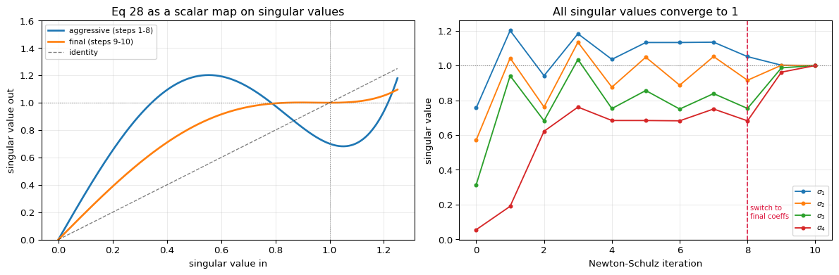
This is a matrix polynomial that acts on each singular value independently — if $\sigma$ is a singular value of $M_{k-1}$, then $a\sigma + b\sigma^3 + c\sigma^5$ is the corresponding singular value of $M_k$. So the whole question is what that scalar map does to values in $[0, 1]$.
DeepSeek's contribution is to use two different coefficient sets:
| steps | $(a, b, c)$ | purpose |
|---|---|---|
| first 8 | $(3.4445,\ -4.7750,\ 2.0315)$ | aggressive — drive singular values toward 1 fast |
| last 2 | $(2,\ -1.5,\ 0.5)$ | gentle — settle them at 1 |
The first polynomial converges quickly but overshoots and oscillates around 1; the second is contractive near 1, so it cleans up the overshoot. Neither is exact — after 10 steps the singular values sit within a few $10^{-4}$ of 1, far below the precision training runs in, which is the whole trade Muon is making. The full algorithm is then:
$$M_t = \mu M_{t-1} + G_t \qquad O'_t = \text{NS}(\mu M_t + G_t) \qquad O_t = O'_t\sqrt{\max(n,m)}\,\gamma \qquad W_t = W_{t-1}(1-\eta\lambda) - \eta O_t$$
with the Nesterov look-ahead $\mu M_t + G_t$ fed to the orthogonaliser, and the $\sqrt{\max(n,m)}$ rescaling chosen so AdamW's learning rates can be reused.
==============================================================================
  MUON: ORTHOGONALISING THE UPDATE (EQ 28)
==============================================================================

Eq 28 acts on each singular value independently
==============================================================================
  If sigma is a singular value of M, then a*s + b*s^3 + c*s^5 is the
  singular value of the next iterate. The matrix polynomial IS a
  scalar map, applied to the spectrum.

    sigma    aggressive       final
  ---------------------------------
     0.01        0.0344      0.0200
     0.10        0.3397      0.1985
     0.30        0.9094      0.5607
     0.60        1.1933      0.9149
     0.90        0.8187      1.0017
     1.00        0.7010      1.0000
  ---------------------------------
  Note both map 1.0 -> 1.0 exactly: 3.4445-4.7750+2.0315 = 0.7010, and 2-1.5+0.5 = 1.0
  A tiny sigma=0.01 is amplified 3.4x per aggressive step - that is
  how near-zero directions get pulled up to 1.

The hybrid schedule, on a real gradient matrix
==============================================================================
  G is (6 x 4). After M/||M||_F the spectrum is
    [0.7558 0.5716 0.3146 0.0553]   (spread 13.7x)

   step       coeffs  singular values
  ----------------------------------------------------------
      0            -  [0.7558 0.5716 0.3146 0.0553]
      1   aggressive  [1.2011 1.0427 0.9412 0.1898]
      2   aggressive  [0.9414 0.7612 0.6823 0.6216]
      3   aggressive  [1.1828 1.1339 1.035  0.7609]
      4   aggressive  [1.0355 0.8756 0.7522 0.6837]
      5   aggressive  [1.1324 1.0479 0.8561 0.6836]
      6   aggressive  [1.1326 0.887  0.7496 0.6819]
      7   aggressive  [1.1343 1.0516 0.8384 0.7498]
      8   aggressive  [1.0513 0.9154 0.753  0.6818]
      9        final  [1.0018 1.0016 0.9866 0.9619]
     10        final  [1.0005 1.0001 1.     1.    ]
  ----------------------------------------------------------

Verify against the exact answer from an SVD
==============================================================================
  exact U V^T singular values : [1. 1. 1. 1.]
  Newton-Schulz after 10 steps: [1.0005 1.0001 1.     1.    ]
  max|NS - U V^T| = 3.78e-04

  This is NOT exact, and is not meant to be. Ten matrix polynomials
  approximate U V^T; an exact answer would need the SVD that Muon is
  avoiding. The question is whether 3.8e-04 is small enough:
    largest singular value off by 5.4e-04
    bf16 resolution near 1.0     ~ 3.9e-03
    -> the error is 10x below the precision the training
       actually runs in, so it is invisible to the update.
  MATCH within bf16 resolution: True

  Why the last two steps matter - spectrum spread:
    after 8 aggressive steps : 3.694e-01
    after 2 final steps      : 5.366e-04

Algorithm 1, one full Muon step
==============================================================================
  momentum  M_t = mu M + G          ||M|| = 4.3120
  Nesterov  mu M_t + G              ||.|| = 8.4083
  orthogonalised O'                 ||O'||= 2.0003
  rescale   x sqrt(max(n,m)) x gamma = x 0.4899
  update    W(1-eta*lam) - eta*O
    ||W|| before 2.7777 -> after 2.7644

  The point of orthogonalising: the raw gradient has RMS 0.8802
  concentrated in its top directions, while the update has RMS
  0.2000 spread evenly across all of them.
8. Putting the efficiency claim back together
Section 1 opened with the KV cache of a BF16 GQA-8 baseline at one million tokens. Now every piece needed to rebuild DeepSeek's side of that comparison is on the table:
- CSA stores $n/4$ entries, HCA stores $n/128$, interleaved across the layers
- each entry is one vector of width $c = 512$, shared by all 64 heads (MQA), not one per head
- there is no separate value cache — the entry is both key and value
- storage is mixed precision: BF16 for the 64 RoPE dimensions, FP8 for the other 448
The last point is easy to skip past and worth a sentence: FP8 halves the cost of 88% of each entry, which is where the "nearly half" saving in the paper comes from.
==============================================================================
  REBUILDING THE ~2% KV CACHE CLAIM
==============================================================================

Baseline: BF16 GQA-8, head dim 128, per layer
==============================================================================
  keys + values, 8 kv-heads x 128 dims x 2 B = 4,096 B/token/layer
  x 1,000,000 x 43 layers = 164.0 GiB

DeepSeek-V4: bytes per compressed entry
==============================================================================
  64 RoPE dims in BF16  =  128 B
  448 other dims in FP8   =  448 B
  total per entry            =  576 B   (vs 1024 B if all BF16 -> 56%)
  and ONE entry serves all 64 heads, as key and as value.

Per layer, at 1M context
==============================================================================
  CSA layer:   250,000 entries x 576 B =    0.134 GiB
  HCA layer:     7,812 entries x 576 B =    0.004 GiB

Whole model: 2 sliding-window layers, then CSA/HCA interleaved
==============================================================================
  20 CSA layers + 21 HCA layers + 2 SWA layers
    CSA total =     2.68 GiB
    HCA total =     0.09 GiB
    SWA total =  0.00014 GiB  (negligible)
    ---------------------------
    DeepSeek-V4 =   2.77 GiB
    baseline    =  164.0 GiB

  ratio = 1.7% of the BF16 GQA-8 baseline
  The paper states 'approximately 2%'. This reconstruction gives 1.7%,
  which lands on the claim using only the numbers stated in the report.

  Caveat worth stating: the per-layer CSA/HCA split is an even
  interleave inferred from 'used in an interleaved manner'. The paper
  does not give the exact per-layer assignment, so treat 1.7% as a
  reconstruction of the right magnitude, not a reproduction.
9. What to take away
The three mechanisms are answers to three different pressures, and it is worth separating them:
mHC is about depth. Widening the residual stream helps, but only if the mixing matrix cannot amplify. Constraining $B_l$ to doubly stochastic makes the map provably non-expansive and — because the Birkhoff polytope is closed under multiplication — keeps it non-expansive at any depth. Sinkhorn–Knopp is just the projection that gets you there, 20 iterations per layer.
CSA and HCA are about context length. Both compress KV entries by pooling with a learned per-channel softmax. CSA compresses gently ($1/4$, overlapped) and then selects with a cheap ReLU-based indexer; HCA compresses hard ($1/128$) and attends densely because there is so little left. Interleaving them gives a fine sparse view and a coarse dense view of the same million tokens.
Muon is about the optimiser. Orthogonalising the update equalises the singular values so no direction dominates, and hybrid Newton–Schulz gets there in 10 matrix polynomials instead of an SVD.
The details in section 5 are not decoration. Shared key/value halves the cache but leaks absolute position, which forces the $\text{RoPE}(-i)$ correction on outputs. Compression creates a local blind spot, which forces the sliding-window branch. Softmax forces every head to attend somewhere, which the attention sink undoes. Each one exists because the mechanism before it broke something.
Verified in this notebook
- Hyper-connections reduce exactly to $x + F(x)$ at $n_{\text{hc}}=1$
- Sinkhorn–Knopp converges to doubly stochastic, $\|B\|_2 = 1$ exactly, and stays so through 43 layers of products
- CSA compression by hand matches the array computation; overlap gives $1/m$, not $1/2m$
- The lightning indexer's top-$k$ matches a brute-force ranking
- $\text{RoPE}(-i)$ after $\text{RoPE}(j)$ depends only on $j-i$ — to $10^{-17}$
- Newton–Schulz after 10 steps matches $UV^T$ from an exact SVD
- The KV cache reconstruction lands on the paper's ~2% claim
Source
Everything above follows DeepSeek-AI, DeepSeek-V4: Towards Highly Efficient Million-Token Context Intelligence, arXiv:2606.19348, 26 April 2026. Equation numbers match the report. Where the report leaves something unspecified — the exact per-layer CSA/HCA assignment — that is flagged in the text rather than guessed silently.
References
- DeepSeek-V4: Towards Highly Efficient Million-Token Context Intelligence
- Hyper-Connections
- Manifold-Constrained Hyper-Connections
- Muon: An optimizer for the hidden layers of neural networks
- DeepSeekMoE: Towards Ultimate Expert Specialization
- Efficient Streaming Language Models with Attention Sinks