🎯 Evaluation Metrics
Every other walkthrough in this series prints an accuracy at some point. This one explains why that number is often close to meaningless, and what to use instead.
The setting that makes it matter is the one you actually have in medical data: class imbalance. Suppose 5% of EEG epochs contain a seizure. A model that outputs "no seizure" for every single epoch — a model containing no information whatsoever — scores 95% accuracy.
$$\text{accuracy} = \frac{\text{correct}}{\text{total}}$$
The formula is not wrong. It is answering a question nobody asked, because it weights a missed seizure and a false alarm identically, and it lets the majority class dominate.
Everything below is computed by hand on 20 epochs, small enough that every prediction can be listed, then checked against scikit-learn.
Display helpers ready: banner, step, check, expand, show_matrix, show_matmul, show_elementwise.
1. A Deliberately Imbalanced Problem
20 EEG epochs, 4 of which contain a seizure. A model has produced a score for each — a probability, not yet a decision.
Keep the two things separate in your head, because the whole notebook turns on it:
- the score is what the model produces,
- the prediction is what you get after choosing a threshold.
The threshold is your decision, not the model's.
20 epochs: 4 seizures, 16 non-seizures (20% positive)

   id   true         label   model score
----------------------------------------
  e19      1       SEIZURE          0.95
  e18      1       SEIZURE          0.83
  e15      0        normal          0.71
  e17      1       SEIZURE          0.68
  e14      0        normal          0.63
  e13      0        normal          0.58
  e12      0        normal          0.52
  e11      0        normal          0.45
  e16      1       SEIZURE          0.44
  e10      0        normal          0.40
  e09      0        normal          0.35
  e08      0        normal          0.31
  e07      0        normal          0.26
  e06      0        normal          0.21
  e05      0        normal          0.18
  e04      0        normal          0.14
  e03      0        normal          0.11
  e02      0        normal          0.08
  e01      0        normal          0.05
  e00      0        normal          0.02
----------------------------------------
(sorted by score, highest first - a good model puts seizures at the top)


the trivial model: predict 'normal' for everything

   correct: 16 of 20
   accuracy = 16/20 = 0.8000  ->  80%
   seizures found: 0 of 4

80% accuracy, and it would never once raise the alarm.
On real EEG data at 1% prevalence the same model scores 99%.
2. The Confusion Matrix
Accuracy collapses four distinct outcomes into one number. Keeping them separate is the whole of evaluation:
| predicted positive | predicted negative | |
|---|---|---|
| actually positive | TP — correct alarm | FN — missed seizure |
| actually negative | FP — false alarm | TN — correct silence |
The two errors are not interchangeable. A false negative is a seizure that went undetected. A false positive is a nurse checking a patient who is fine. Any single metric has already made an assumption about their relative cost — usually silently.
threshold = 0.5

   id    score   pred   true                     outcome
--------------------------------------------------------
  e19     0.95      1      1           TP  correct alarm
  e18     0.83      1      1           TP  correct alarm
  e15     0.71      1      0             FP  FALSE ALARM
  e17     0.68      1      1           TP  correct alarm
  e14     0.63      1      0             FP  FALSE ALARM
  e13     0.58      1      0             FP  FALSE ALARM
  e12     0.52      1      0             FP  FALSE ALARM
  e11     0.45      0      0         TN  correct silence
  e16     0.44      0      1          FN  MISSED SEIZURE
  e10     0.40      0      0         TN  correct silence
  e09     0.35      0      0         TN  correct silence
  e08     0.31      0      0         TN  correct silence
  e07     0.26      0      0         TN  correct silence
  e06     0.21      0      0         TN  correct silence
  e05     0.18      0      0         TN  correct silence
  e04     0.14      0      0         TN  correct silence
  e03     0.11      0      0         TN  correct silence
  e02     0.08      0      0         TN  correct silence
  e01     0.05      0      0         TN  correct silence
  e00     0.02      0      0         TN  correct silence
--------------------------------------------------------


confusion matrix

                      pred POSITIVE    pred NEGATIVE
------------------------------------------------------
   actual POSITIVE           TP = 3           FN = 1
   actual NEGATIVE           FP = 4          TN = 12
------------------------------------------------------
   TP + FP + FN + TN = 20  (= n = 20): True

accuracy = (TP + TN) / n = (3 + 12) / 20 = 0.7500
trivial model accuracy   = 0.8000

So this model is WORSE than predicting 'normal' every time, by accuracy alone -
even though it correctly found 3 of the 4 seizures. Accuracy is
punishing it for the 4 false alarms and giving no credit for the
detections, because 16 negatives dominate the arithmetic.
3. Precision, Recall, and $F_1$
Three metrics, each asking a different question. Notice what each one ignores.
$$\text{precision} = \frac{TP}{TP+FP} \qquad\text{"when it alarms, how often is it right?"}$$
$$\text{recall} = \frac{TP}{TP+FN} \qquad\text{"of the real seizures, how many were caught?"}$$
$$F_1 = 2\cdot\frac{\text{precision}\cdot\text{recall}}{\text{precision}+\text{recall}}$$
Neither precision nor recall uses TN. That is precisely why they survive imbalance — the huge, easy negative class cannot inflate them.
$F_1$ is the harmonic mean, not the arithmetic one, and that choice matters: the harmonic mean is dominated by the smaller value, so a model cannot score well by maximising one metric and abandoning the other.
at threshold 0.5:  TP=3  FP=4  FN=1  TN=12

   precision   = TP/(TP+FP) = 3/(3+4) = 3/7 = 0.428571
   recall      = TP/(TP+FN) = 3/(3+1) = 3/4 = 0.750000
   specificity = TN/(TN+FP) = 12/(12+4) = 12/16 = 0.750000

   F1 = 2 * (0.4286 * 0.7500) / (0.4286 + 0.7500)
      = 2 * 0.321429 / 1.178571 = 0.545455

   arithmetic mean of precision and recall = 0.589286
   harmonic mean (F1)                       = 0.545455
   the harmonic mean is lower - it always is, unless the two are equal


why the harmonic mean: a model that alarms on EVERYTHING

   precision = 4/20 = 0.2000   recall = 1.0000
   arithmetic mean = 0.6000   <- looks respectable
   F1 (harmonic)   = 0.3333   <- correctly poor

   The arithmetic mean lets a useless model hide behind perfect recall.
   The harmonic mean does not.


the trivial 'always normal' model under each metric:

        metric    trivial model    our model
--------------------------------------------
      accuracy           0.8000       0.7500
     precision    0 (undefined)       0.4286
        recall           0.0000       0.7500
            F1           0.0000       0.5455
--------------------------------------------

Accuracy ranks the useless model HIGHER. Every other metric ranks it
at zero, which is the correct answer.
4. The Threshold Is a Choice
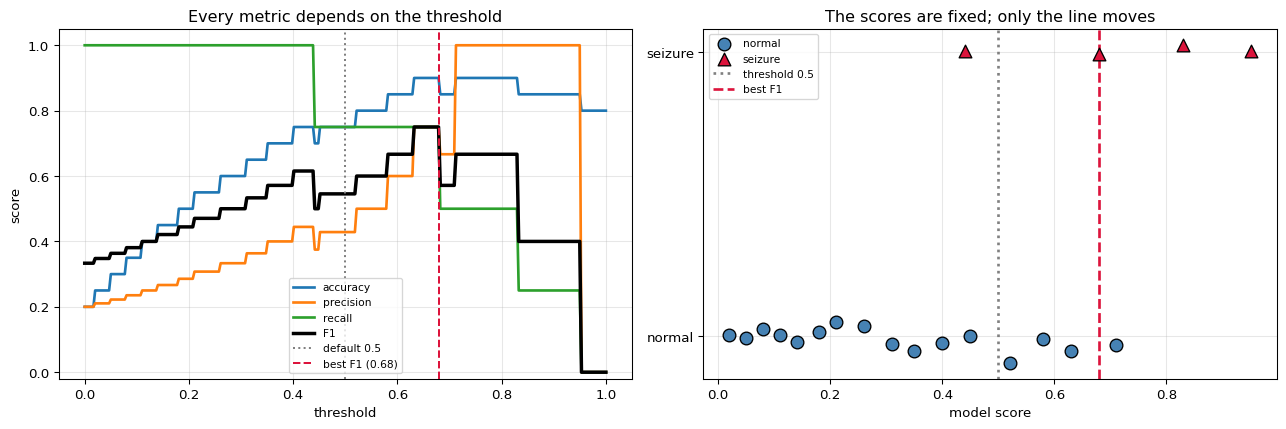
The model produced scores. Turning a score into a decision requires a cut-off, and that cut-off is a policy decision, not a property of the model.
Lower it and you catch more seizures but raise more false alarms. Raise it and alarms become trustworthy but seizures slip through. Nothing about the model changes — the scores are fixed. Only the line moves.
threshold   TP   FP   FN   TN   accuracy   precision    recall        F1
--------------------------------------------------------------------------
      0.00    4   16    0    0     0.2000      0.2000    1.0000    0.3333
      0.15    4   11    0    5     0.4500      0.2667    1.0000    0.4211
      0.30    4    8    0    8     0.6000      0.3333    1.0000    0.5000
      0.42    4    5    0   11     0.7500      0.4444    1.0000    0.6154
      0.50    3    4    1   12     0.7500      0.4286    0.7500    0.5455
      0.60    3    2    1   14     0.8500      0.6000    0.7500    0.6667
      0.70    2    1    2   15     0.8500      0.6667    0.5000    0.5714
      0.90    1    0    3   16     0.8500      1.0000    0.2500    0.4000
      1.01    0    0    4   16     0.8000      0.0000    0.0000    0.0000
--------------------------------------------------------------------------

read the extremes:
   threshold 0.00 - alarm on everything: recall 1.00, precision 0.20
   threshold 1.01 - never alarm        : recall 0.00, precision undefined

Everything useful is in between, and where you sit is a decision about
which error you can tolerate.

threshold maximising F1: 0.680  (F1 = 0.7500)
the DEFAULT threshold of 0.5 gives F1 = 0.5455

Moving one number - with no retraining at all - improves F1 by +0.2045.
0.5 is a convention inherited from balanced problems, not a good default
for imbalanced ones.
Right panel: one seizure (e16) scored 0.44 and sits among the negatives.
No threshold separates the classes perfectly here - moving the line just
trades one error type for the other.
5. ROC and AUC
Rather than pick one threshold, sweep all of them and plot the result. The ROC curve plots:
$$\text{TPR (recall)} = \frac{TP}{TP+FN} \qquad\text{against}\qquad \text{FPR} = \frac{FP}{FP+TN}$$
AUC is the area under that curve, and it has an interpretation that makes it worth knowing:
AUC is the probability that a randomly chosen positive scores higher than a randomly chosen negative.
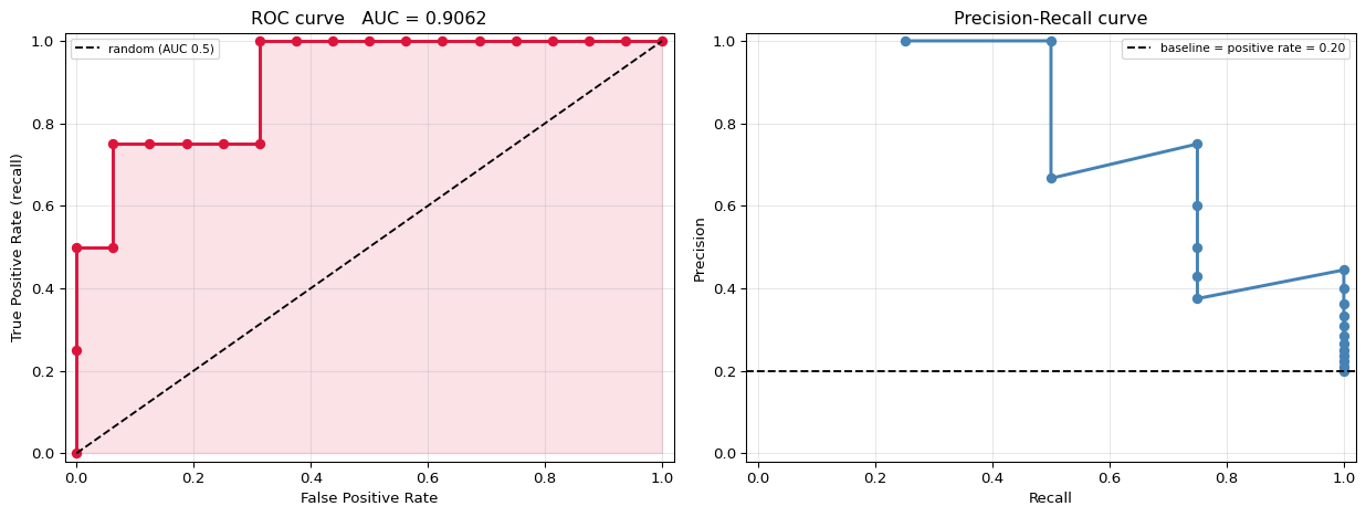
So AUC = 0.5 is a coin flip and AUC = 1.0 is perfect separation. Crucially it is threshold-free — it measures the ranking, not any particular decision. That interpretation is verified below by counting pairs directly.
building the ROC curve by walking down the sorted scores

 rank     id    score   true   TP   FP       TPR       FPR
--------------------------------------------------------------
    1    e19     0.95      1    1    0    0.2500    0.0000  <- step UP  (a positive)
    2    e18     0.83      1    2    0    0.5000    0.0000  <- step UP  (a positive)
    3    e15     0.71      0    2    1    0.5000    0.0625  <- step RIGHT (a negative)
    4    e17     0.68      1    3    1    0.7500    0.0625  <- step UP  (a positive)
    5    e14     0.63      0    3    2    0.7500    0.1250  <- step RIGHT (a negative)
    6    e13     0.58      0    3    3    0.7500    0.1875  <- step RIGHT (a negative)
    7    e12     0.52      0    3    4    0.7500    0.2500  <- step RIGHT (a negative)
    8    e11     0.45      0    3    5    0.7500    0.3125  <- step RIGHT (a negative)
    9    e16     0.44      1    4    5    1.0000    0.3125
   10    e10     0.40      0    4    6    1.0000    0.3750
   11    e09     0.35      0    4    7    1.0000    0.4375
   12    e08     0.31      0    4    8    1.0000    0.5000
   13    e07     0.26      0    4    9    1.0000    0.5625
   14    e06     0.21      0    4   10    1.0000    0.6250
   15    e05     0.18      0    4   11    1.0000    0.6875
   16    e04     0.14      0    4   12    1.0000    0.7500
   17    e03     0.11      0    4   13    1.0000    0.8125
   18    e02     0.08      0    4   14    1.0000    0.8750
   19    e01     0.05      0    4   15    1.0000    0.9375
   20    e00     0.02      0    4   16    1.0000    1.0000
--------------------------------------------------------------

AUC by trapezoidal area under the curve: 0.906250

AUC by counting pairs:
   positive-negative pairs      : 4 x 16 = 64
   pairs where positive > negative: 58
   ties (counted as half)        : 0
   AUC = (58 + 0.5*0) / 64 = 0.906250

   trapezoid vs pair-counting MATCH: True

The two definitions agree exactly, which is the point: AUC really is
'how often does the model rank a seizure above a non-seizure'.
Why the PR curve is the better one here
ROC has a weakness on imbalanced data, and it comes straight from the FPR formula:
$$\text{FPR} = \frac{FP}{FP+TN}$$
With 16 negatives and 4 positives, going from 0 to 4 false alarms moves FPR by only $4/16 = 0.25$. With 10 000 negatives it would move it by 0.0004 — invisible. The enormous $TN$ count in the denominator hides false alarms.
Precision has no $TN$:
$$\text{precision} = \frac{TP}{TP+FP}$$
so 4 false alarms against 4 true detections halves it, whatever the negative count. On imbalanced problems the precision-recall curve is the more honest picture, and its baseline is the positive rate rather than 0.5.
the same model at four operating points

 threshold    recall   precision       FPR           what it means in practice
------------------------------------------------------------------------------
      0.20    1.0000      0.2857    0.6250  catch nearly everything, many alarms
      0.44    1.0000      0.4444    0.3125                catch all 4 seizures
      0.50    0.7500      0.4286    0.2500                         the default
      0.80    0.5000      1.0000    0.0000           only alarm when very sure
------------------------------------------------------------------------------

The ROC and PR curves contain the SAME information - both are just the
score ranking, re-plotted. But PR makes the cost of false alarms visible
at a glance, and ROC does not when negatives vastly outnumber positives.
6. Choosing a Threshold From Costs
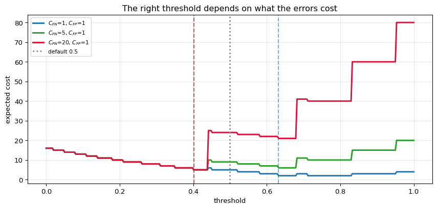
Once you accept that the threshold is a decision, it can be made properly — by stating what the errors cost.
$$\text{expected cost} = C_{FN}\cdot FN \;+\; C_{FP}\cdot FP$$
For seizure detection a missed event is far worse than a false alarm. If a miss costs 20 and an alarm costs 1, the optimal threshold is well below 0.5 — and it falls out of arithmetic instead of habit.
C_FN    C_FP   best thr   TP   FP   FN     cost   cost at 0.5    saving
--------------------------------------------------------------------------
     1       1      0.632    3    1    1        2             5         3
     5       1      0.401    4    5    0        5             9         4
    20       1      0.401    4    5    0        5            24        19
    50       1      0.401    4    5    0        5            54        49
     1       5      0.712    2    0    2        2            21        19
--------------------------------------------------------------------------

As the cost of a miss rises, the optimal threshold falls - the model is
told to become more willing to alarm. Note the last row: when false
alarms are the expensive error, the threshold goes UP instead.

None of this requires retraining. The model produced a ranking; the
threshold turns that ranking into a policy, and the policy should come
from the costs.
7. Regression Metrics, Briefly
For continuous targets the same principle applies — each metric encodes an assumption about which errors matter.
| Metric | Formula | Character |
|---|---|---|
| MSE | $\frac{1}{n}\sum(y-\hat y)^2$ | punishes large errors hardest; units squared |
| RMSE | $\sqrt{\text{MSE}}$ | same, back in the original units |
| MAE | $\frac{1}{n}\sum\lvert y-\hat y\rvert$ | every error counts linearly; outlier-tolerant |
| $R^2$ | $1 - SS_{res}/SS_{tot}$ | relative to predicting the mean |
| MAPE | $\frac{100}{n}\sum\lvert\frac{y-\hat y}{y}\rvert$ | percentage; breaks when $y \approx 0$ |
two models with the SAME total absolute error

  id        y    model A     err A    model B     err B
----------------------------------------------------
   0      2.0        2.5     -0.50        2.0      0.00
   1      4.0        4.5     -0.50        4.0      0.00
   2      6.0        6.5     -0.50        6.0      0.00
   3      8.0        8.5     -0.50        8.0      0.00
   4     10.0       10.5     -0.50       10.0      0.00
   5     12.0       12.5     -0.50       15.0     -3.00
----------------------------------------------------
|sum|                          3.00                 3.00

    metric      model A      model B    prefers
----------------------------------------------
       MAE       0.5000       0.5000          B
       MSE       0.2500       1.5000          A
      RMSE       0.5000       1.2247          A
       R^2       0.9786       0.8714          A
----------------------------------------------

MAE calls them equal (0.50 vs 0.50). MSE strongly prefers A, because
one error of 3 costs 9 while six errors of 0.5 cost 1.5 in total.

Neither is right. If one large miss is much worse than several small
ones - a spike detector, say - use MSE. If they are equally bad, use MAE.
8. Checking Against scikit-learn
confusion matrix (sklearn order: [[TN, FP], [FN, TP]])

   sklearn : [[12, 4], [1, 3]]
   ours    : [[12, 4], [1, 3]]
   MATCH: True

        metric          ours       sklearn    match
--------------------------------------------------
      accuracy    0.75000000    0.75000000     True
     precision    0.42857143    0.42857143     True
        recall    0.75000000    0.75000000     True
            F1    0.54545455    0.54545455     True
AUC (trapezoid)    0.90625000    0.90625000     True
   AUC (pairs)    0.90625000    0.90625000     True
--------------------------------------------------

ROC curve points
   ours    : 21 points
   sklearn : 8 points  (it de-duplicates equal thresholds)
   every sklearn point is on our curve: True


regression metrics

    metric          ours       sklearn    match
----------------------------------------------
       MSE    0.25000000    0.25000000     True
       MAE    0.50000000    0.50000000     True
       R^2    0.97857143    0.97857143     True
----------------------------------------------


threshold-free scores on the imbalanced problem

   ROC AUC          : 0.906250
   Average Precision: 0.798611  (area under PR)
   baseline AP      : 0.200000  (= the positive rate)

   ROC AUC looks strong; AP is more modest. On imbalanced data that gap
   is normal, and AP is the number to trust.
9. Summary
| Metric | Formula | Uses TN? | Use it when |
|---|---|---|---|
| Accuracy | $(TP+TN)/n$ | yes | classes are balanced and errors cost the same |
| Precision | $TP/(TP+FP)$ | no | false alarms are expensive |
| Recall | $TP/(TP+FN)$ | no | misses are expensive |
| $F_1$ | harmonic mean | no | you need one number and both errors matter |
| Specificity | $TN/(TN+FP)$ | yes | the negative class matters in its own right |
| ROC AUC | area under TPR–FPR | yes | comparing rankings, roughly balanced data |
| Average Precision | area under PR | no | imbalanced data |
The one idea: a classifier does not output a class, it outputs a ranking. Metrics that summarise the ranking (AUC, AP) measure the model. Metrics that summarise one threshold (accuracy, precision, recall, $F_1$) measure the model plus a policy you chose — and 0.5 is a convention, not a choice.
The trap to remember: at 5% prevalence, a model that always says "no" scores 95% accuracy and zero on everything else. Whenever an accuracy is quoted without the class balance beside it, the number cannot be interpreted.
What is deliberately left out: multi-class averaging (macro, micro, weighted), Cohen's kappa and Matthews correlation, calibration and reliability diagrams — a model can rank perfectly and still have badly wrong probabilities — and the evaluation of ranking and detection tasks, where a "correct" detection needs a definition of overlap.