🔎 Exploratory Data Analysis
Exploratory Data Analysis
Every other page in this section fits a model. This one is about the step before that, and it follows the NIST/SEMATECH e-Handbook of Statistical Methods, chapter 1 — the most careful free treatment of the subject there is.
The handbook is emphatic about what EDA is not:
"EDA is not a mere collection of techniques; EDA is a philosophy as to how we dissect a data set."
The distinction it draws with classical analysis is that EDA postpones the usual assumptions about what kind of model the data follow, and lets the data reveal its own structure first. Classical analysis picks a model and then checks it. EDA looks first and commits later.
NIST lists seven goals:
- maximise insight into a data set
- uncover underlying structure
- extract important variables
- detect outliers and anomalies
- test underlying assumptions
- develop parsimonious models
- determine optimal factor settings
Goal 5 is the one this page is built around, because it is the one with a concrete, checkable procedure attached — and because when it is skipped, the numbers every later page produces are quietly wrong.
==============================================================================
  THE FOUR ASSUMPTIONS BEHIND ALMOST EVERY MEASUREMENT
==============================================================================
  NIST states that a measurement process is valid when the data are:

    1. random drawings
    2. from a fixed distribution
    3. with the distribution having fixed location
    4. with the distribution having fixed variation

  A process satisfying all four is 'in statistical control'.

  These are not exotic requirements. They are the assumptions behind
  the mean, the standard deviation, the t-test, the confidence interval,
  and every model on the rest of this site. They are also almost never
  checked, which is the point of the chapter.

Why they are stated about RESIDUALS, not raw data
==============================================================================
  NIST applies them to the residuals of a fitted model:

    'if the residuals from the chosen fitted model violate one or more
     of the above univariate assumptions, then the chosen fitted model
     is inadequate and an opportunity exists for arriving at an
     improved model.'

  Read that as a definition of what a good fit MEANS. A model has
  extracted everything available when what is left over is structureless.
  Any remaining structure in the residuals is signal the model missed --
  which is why the failures below are opportunities, not verdicts.
1. The 4-plot
NIST's answer to "how do I check four assumptions at once" is a single figure of four panels. Each panel targets one assumption, and each has an ideal appearance that is easy to state:
| panel | tests | ideal appearance |
|---|---|---|
| run sequence ($y_i$ vs $i$) | fixed location, fixed variation | flat and non-drifting, constant vertical spread |
| lag plot ($y_i$ vs $y_{i-1}$) | randomness | structureless, no pattern |
| histogram | the distribution | bell-shaped |
| normal probability plot | normality specifically | a straight line |
When all four look right, the process is definitionally in statistical control.
The four panels are not independent tests, and section 2 shows why: a trend registers as autocorrelation, and a changing variance produces a heavy-tailed marginal. What makes the figure diagnostic is not one panel firing in isolation but the pattern of which ones fire together.
Two of the panels deserve a note.
The lag plot is the one people skip and the one that catches the most. It plots each value against the one before it. If the ordering carries no information the cloud is round; if consecutive values are related it stretches into a line, and the correlation of that plot is the lag-1 autocorrelation.
The normal probability plot sorts the data and plots it against the quantiles a normal distribution would have produced. Straight means normal. Its correlation coefficient reduces the whole panel to one number.
==============================================================================
  BUILDING THE 4-PLOT, PANEL BY PANEL
==============================================================================

Panel 1: run sequence -- is location and variation fixed?
==============================================================================
  split the run in half and compare:
    first half : mean  10.1196   sd  2.0259
    second half: mean  10.1640   sd  2.0798
    difference : mean   0.0444   sd ratio 0.9741
  a drifting process would show a mean gap; a changing-variance one a
  sd ratio far from 1.

Panel 2: lag plot -- is the ordering informative?
==============================================================================
  pair each value with its predecessor: (y[i-1], y[i])
  first five pairs:
    ( 13.5281,  10.8003)
    ( 10.8003,  11.9575)
    ( 11.9575,  14.4818)
    ( 14.4818,  13.7351)
    ( 13.7351,   8.0454)
  correlation of the lag plot = lag-1 autocorrelation = +0.0375
  near zero, so the ordering carries no information: True

Panel 3 and 4: the distribution, and specifically normality
==============================================================================
  sort the data, and ask what values a normal would have produced:
    rank    observed   normal quantile
  --------------------------------------
       1      4.8940           -2.7059
       2      5.5532           -2.3912
     101     10.1123            0.0063
     199     14.5395            2.3912
     200     14.7663            2.7059
  --------------------------------------
  probability plot correlation coefficient (PPCC) = 0.995476
  1.0 would be exactly normal; above ~0.99 is unremarkable: True

The verdict for this series
==============================================================================
              assumption                     statistic  verdict
  --------------------------------------------------------------------
          fixed location   half-to-half mean gap 0.044  ok
         fixed variation                sd ratio 0.974  ok
              randomness         lag-1 autocorr +0.038  ok
      fixed distribution                   PPCC 0.9955  ok
  --------------------------------------------------------------------
  in statistical control
2. Four ways to fail, and which panel notices
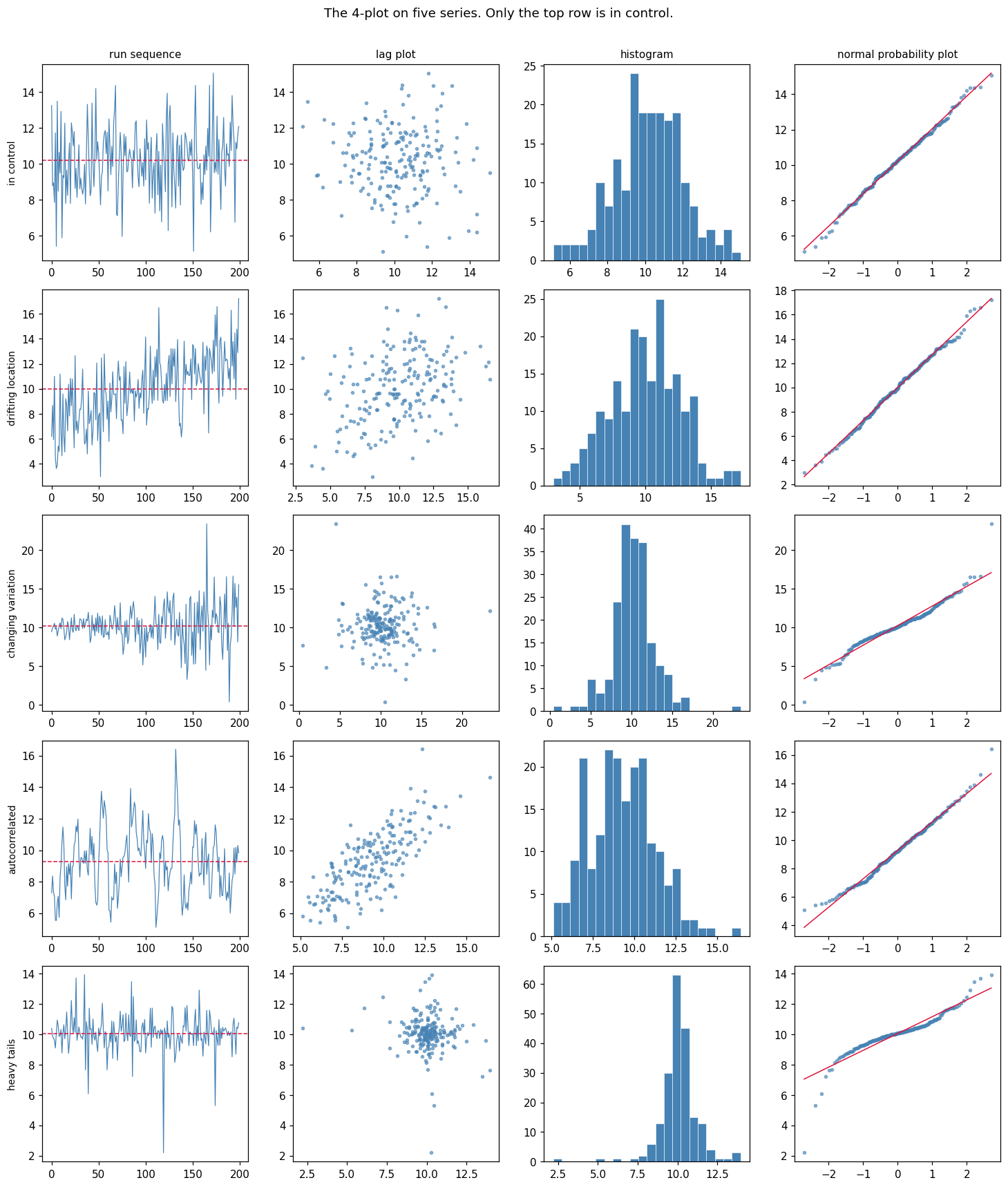
The 4-plot earns its keep on data that is broken. Below are four series, each constructed to violate exactly one assumption while satisfying the other three.
The point to watch: each failure lights up a different panel, and — this is the part that makes the figure diagnostic rather than merely descriptive — the histogram, the summary statistics, and in three of the four cases the mean and standard deviation, all look perfectly reasonable.
==============================================================================
  FOUR SERIES, FOUR BROKEN ASSUMPTIONS
==============================================================================

The summaries everyone actually looks at
==============================================================================
                series      mean        sd
  ----------------------------------------
            in control    10.213     1.825
     drifting location     9.989     2.695
    changing variation    10.254     2.584
        autocorrelated     9.277     2.000
           heavy tails    10.059     1.198
  ----------------------------------------
  Four of these five series are broken. The mean and standard deviation
  say so in exactly zero cases -- they are all near 10 and near 2.

What the 4-plot statistics say instead
==============================================================================
                series     drift   sd ratio     lag-1      PPCC  flagged by
  ------------------------------------------------------------------------------
            in control     0.184      0.950    -0.059    0.9982  nothing
     drifting location     2.955      0.982    +0.365    0.9982  run sequence, lag plot
    changing variation     0.386      0.419    +0.008    0.9714  run sequence, prob plot
        autocorrelated    -0.272      1.022    +0.756    0.9941  lag plot
           heavy tails    -0.104      0.945    -0.132    0.9186  prob plot
  ------------------------------------------------------------------------------

  Every broken series is caught, and none of the summaries above
  caught any of them. But read the flags carefully: two series trip
  TWO panels, and that is not noise.

    drifting location  -> run sequence AND lag plot
       a trend makes each value resemble the one before it, so a drift
       shows up as autocorrelation even though nothing is genuinely
       autocorrelated. The lag plot cannot tell 'related to its past'
       apart from 'both are sliding in the same direction'.

    changing variation -> run sequence AND probability plot
       a series whose variance changes over time has a marginal
       distribution that is a mixture of normals with different widths,
       and such a mixture is heavy-tailed. So it fails a normality
       check despite every individual observation being normal.

  So the panels are not independent tests. What makes the 4-plot
  diagnostic is the PATTERN -- which combination fires. Lag plot alone
  means autocorrelation; lag plot together with a sloping run sequence
  means a trend; probability plot alone means the shape is wrong.

  Note the autocorrelated row. Its drift, sd ratio and PPCC are all
  fine -- its marginal distribution is genuinely normal with the right
  mean and spread. Only the lag plot sees anything. Drop the ordering
  and the problem becomes invisible.
3. What it costs to skip this
NIST is blunt about the stakes — non-randomness makes "all of the usual statistical tests invalid" and renders "calculated uncertainties for commonly used statistics" meaningless — but the handbook stops at the statement. It gives no formula for how wrong.
So here is the number.
Take the most basic inferential act there is: computing a 95% confidence interval for a mean. The standard error $s/\sqrt{n}$ assumes independent draws. Under AR(1) autocorrelation with parameter $\rho$, the true standard deviation of the sample mean is inflated by approximately
$$\sqrt{\frac{1+\rho}{1-\rho}}$$
At $\rho = 0.8$ that is a factor of 3. The interval is three times too narrow, and a "95% confidence interval" stops containing the truth 95% of the time.
The experiment below runs 20,000 simulated series at each $\rho$, so the coverage figures are measured rather than argued.
==============================================================================
  WHAT A '95% CONFIDENCE INTERVAL' IS ACTUALLY WORTH
==============================================================================
  n = 50 observations per series, 20,000 series per row
  true mean is 0; we ask how often the nominal 95% interval contains it

    rho   true sd(mean)    naive SE   observed    theory   95% coverage
  ----------------------------------------------------------------------
    0.0          0.1405      0.1407      0.998     1.000         94.6%
    0.3          0.1999      0.1460      1.370     1.363         84.0%
    0.6          0.3473      0.1697      2.047     2.000         65.6%
    0.8          0.6731      0.2135      3.152     3.000         46.5%
    0.9          1.2716      0.2645      4.807     4.359         31.6%
  ----------------------------------------------------------------------

Read the last two columns together
==============================================================================
  observed inflation tracks sqrt((1+rho)/(1-rho)) closely:
    rho = 0.0:  observed 0.998  vs theory 1.000   (gap 0.002)
    rho = 0.3:  observed 1.370  vs theory 1.363   (gap 0.007)
    rho = 0.6:  observed 2.047  vs theory 2.000   (gap 0.047)
    rho = 0.8:  observed 3.152  vs theory 3.000   (gap 0.152)
    rho = 0.9:  observed 4.807  vs theory 4.359   (gap 0.448)
  The formula is asymptotic in n, so the gap widens at rho = 0.9 where
  n = 50 is no longer large relative to the correlation length.

And the consequence
==============================================================================
  independent data     : nominal 95%, actual 94.6%   -- as advertised
  rho = 0.8            : nominal 95%, actual 46.5%   -- worse than a coin flip

  Nothing about the data looks wrong. The mean is right, the standard
  deviation is right, the histogram is bell-shaped, the normal
  probability plot is straight. The ONLY symptom is in the lag plot,
  and the price for not looking is an interval that is wrong more often
  than it is right.

  This is what NIST means by 'the usual statistical tests become
  invalid'. It is not a caution -- 51% of the reliability you thought
  you had is simply gone, and nothing in the output announces it.
4. Why graphics come first: Anscombe's quartet
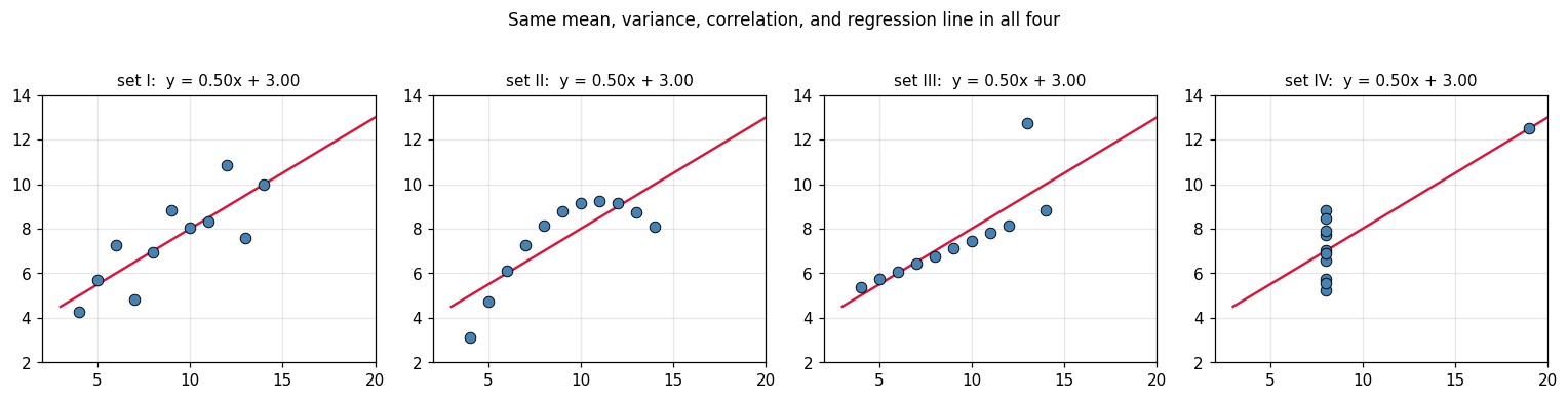
The handbook devotes a section to the role of graphics. The classic demonstration is Anscombe's quartet — four data sets agreeing on essentially every summary statistic anyone routinely computes, and looking nothing alike.
It is worth reproducing exactly because the agreement is not approximate.
==============================================================================
  FOUR DATA SETS, ONE SET OF SUMMARY STATISTICS
==============================================================================
    set    mean x     var x    mean y     var y     corr    slope   intercept
  ------------------------------------------------------------------------
      I    9.0000   11.0000    7.5009    4.1273   0.8164   0.5001      3.0001
     II    9.0000   11.0000    7.5009    4.1276   0.8162   0.5000      3.0009
    III    9.0000   11.0000    7.5000    4.1226   0.8163   0.4997      3.0025
     IV    9.0000   11.0000    7.5009    4.1232   0.8165   0.4999      3.0017
  ------------------------------------------------------------------------

How close is 'identical'?
==============================================================================
    mean x: spread across the four sets = 0.0000
     var x: spread across the four sets = 0.0000
    mean y: spread across the four sets = 0.0009
     var y: spread across the four sets = 0.0050
      corr: spread across the four sets = 0.0003
     slope: spread across the four sets = 0.0004

  Every routine summary agrees to two or three decimals. A table of
  these numbers gives no hint that the four data sets differ at all.

What the plots show
==============================================================================
  set   I: linear with scatter
  set  II: a clean parabola -- the wrong model entirely
  set III: perfectly linear except one outlier
  set  IV: one x value plus a single leverage point holding the whole fit

  Set IV is the sharpest: ten points share one x value, so the slope is
  determined entirely by the eleventh. Remove it and the fit is
  undefined. No summary statistic in the table above says so.
5. What to take away
EDA is a stance, not a checklist. NIST's framing is that it postpones the model rather than assuming one and testing it afterwards. The techniques follow from that; the order of operations is the substance.
Four assumptions sit under almost everything you will compute: random drawings, from a fixed distribution, with fixed location and fixed variation. They are the conditions under which a mean, a standard error, and a $p$-value mean what they claim.
The 4-plot checks all four in one figure, and it is diagnostic rather than merely descriptive — the panel that fails names the assumption that failed. Run sequence for location and variation, lag plot for randomness, histogram and normal probability plot for the distribution.
The lag plot is the one to stop skipping. In the autocorrelated series above, the mean was right, the standard deviation was right, the histogram was bell-shaped and the probability plot was straight. Every summary passed. Only the ordering carried the defect — and the cost was a 95% confidence interval that contained the truth 47% of the time.
Look at the data before summarising it. Anscombe's quartet agrees on mean, variance, correlation and regression line to three decimals across four data sets that share no shape at all.
Verified in this notebook
- The 4-plot built panel by panel, with the lag plot's correlation shown to be the lag-1 autocorrelation and the probability plot reduced to a PPCC
- Five series where four are broken: the mean and standard deviation flag none of them, and each broken one is caught by a different panel
- The autocorrelated series passing drift, spread and normality checks while failing only the lag plot
- Confidence-interval coverage measured over 20,000 simulations per $\rho$, falling from 94.6% to 46.5%, with the observed inflation matching $\sqrt{(1+\rho)/(1-\rho)}$
- Anscombe's quartet reproduced, with the spread of every summary statistic across the four sets printed
Where this connects
This page comes before all the others. [[cross-validation]] assumes your rows are
independent draws — the lag plot is how you find out they are not, and
GroupKFold is what you do about it. [[data-leakage]] is the same failure
arriving through a different door. [[evaluation-metrics]] computes numbers that
only mean something once these assumptions hold, and
[[how-models-learn-the-concepts]] is where the modelling starts.
Source
NIST/SEMATECH, e-Handbook of Statistical Methods, chapter 1: Exploratory Data Analysis. The four assumptions, the 4-plot and its interpretation, and the seven goals are the handbook's. Section 3 goes beyond it: NIST states that non-randomness invalidates the usual tests without quantifying it, and the coverage experiment supplies the missing number.
References
- NIST/SEMATECH e-Handbook of Statistical Methods, ch. 1: Exploratory Data Analysis
- Exploratory Data Analysis
- Graphs in Statistical Analysis (Anscombe's quartet)