🔮 Gaussian Mixtures & EM
The K-Means walkthrough ended on three failures it could not fix: stretched clusters, clusters of very different sizes, and any question of how confident an assignment is.
All three come from the same two restrictions. K-means represents a cluster by a single point, and assigns every sample to exactly one cluster — hard assignment.
A Gaussian mixture removes both. A cluster becomes a full distribution:
$$p(\mathbf{x}) = \sum_{k=1}^{K}\pi_k\,\mathcal{N}(\mathbf{x}\mid\boldsymbol{\mu}_k,\Sigma_k), \qquad \sum_k \pi_k = 1$$
with a mixing weight $\pi_k$ (how large), a mean $\boldsymbol{\mu}_k$ (where), and a covariance $\Sigma_k$ (what shape and orientation). Assignment becomes a probability.
Fitting it uses EM, which is the same alternating pattern as Lloyd's algorithm with one substitution: soft responsibilities instead of hard assignments. In fact k-means is the limiting case, and that is shown numerically at the end.
Display helpers ready: banner, step, check, expand, show_matrix, show_matmul, show_elementwise.
1. The Data
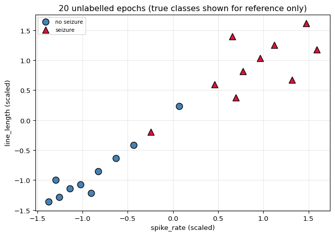
The same 20 EEG epochs as the K-Means walkthrough, with the labels again withheld, so the two methods can be compared directly on identical points.
20 epochs x 2 features, classes [10, 10]

    id   spike_rate   line_length   class         label
-------------------------------------------------------
  ep00          1.0          12.0       0    no seizure
  ep01          1.6          15.0       0    no seizure
  ep02          0.7          11.0       0    no seizure
  ep03          2.1          18.0       0    no seizure
  ep04          1.3          14.0       0    no seizure
  ep05          2.6          21.0       0    no seizure
  ep06          0.9          16.0       0    no seizure
  ep07          1.9          13.0       0    no seizure
  ep08          3.1          24.0       0    no seizure
  ep09          4.4          33.0       0    no seizure
  ep10          6.2          41.0       1       seizure
  ep11          7.1          47.0       1       seizure
  ep12          5.4          38.0       1       seizure
  ep13          8.0          52.0       1       seizure
  ep14          6.7          44.0       1       seizure
  ep15          5.9          49.0       1       seizure
  ep16          7.6          39.0       1       seizure
  ep17          6.0          35.0       1       seizure
  ep18          3.6          27.0       1       seizure
  ep19          8.3          46.0       1       seizure
-------------------------------------------------------

feature means : [ 4.22 29.75]
feature stds  : [ 2.564 13.794]

Note the scales: line_length spans ~41 while spike_rate spans ~8.
Any algorithm that measures DISTANCE will be dominated by the larger one
unless the features are scaled - that matters for KNN and SVM below.
K = 2 components, D = 2 dimensions

parameters per component: 1 weight + 2 mean + 3 covariance = 6
total (minus one, since the weights must sum to 1): 11

k-means, by comparison, has only 4 parameters - just the centres.
2. The Multivariate Gaussian
$$\mathcal{N}(\mathbf{x}\mid\boldsymbol{\mu},\Sigma) = \frac{1}{(2\pi)^{D/2}\lvert\Sigma\rvert^{1/2}} \exp\!\left(-\tfrac{1}{2}(\mathbf{x}-\boldsymbol{\mu})^\top\Sigma^{-1}(\mathbf{x}-\boldsymbol{\mu})\right)$$
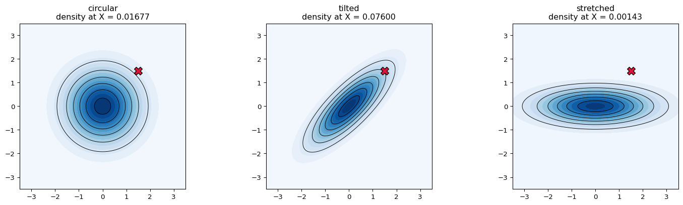
The covariance is what k-means lacks. Its off-diagonal entries let the ellipse tilt; its diagonal lets the axes have different widths. That single matrix is the difference between a circle and an arbitrarily oriented ellipse.
The quadratic form in the exponent is the squared Mahalanobis distance — distance measured in units of the cluster's own spread, so a point far along a wide direction can be closer than one nearer along a narrow direction.
two covariances, same mean

circular (2, 2) =
            0 |   +1.00    +0.00
            1 |   +0.00    +1.00

tilted (off-diagonal 0.8) (2, 2) =
            0 |   +1.00    +0.80
            1 |   +0.80    +1.00

determinants: circular 1.0000, tilted 0.3600


the point [1.5 1.5] under each

   circular:
      Sigma^-1 =
[[1. 0.]
           [0. 1.]]
      Mahalanobis^2 = d^T Sigma^-1 d = 4.500000
      density = exp(-2.2500) / sqrt((2pi)^2 * 1.0000) = 0.01677481
      Euclidean^2 (what k-means uses) = 4.500000

   tilted:
      Sigma^-1 =
[[ 2.7778 -2.2222]
           [-2.2222  2.7778]]
      Mahalanobis^2 = d^T Sigma^-1 d = 2.500000
      density = exp(-1.2500) / sqrt((2pi)^2 * 0.3600) = 0.07599776
      Euclidean^2 (what k-means uses) = 4.500000

Euclidean distance is identical in both cases; the DENSITY is not.
Under the tilted Gaussian this point lies along the direction of high
variance, so it is unremarkable. k-means could never make that
distinction - it has no Sigma.
The red X is the same point in all three. Its density differs by orders
of magnitude - and the density is what decides cluster membership.
3. EM — Soft Assignment
Two steps, alternating, exactly like Lloyd's algorithm.
E-step. Compute the responsibility of component $k$ for point $i$ — the posterior probability that $i$ came from $k$:
$$\gamma_{ik} = \frac{\pi_k\,\mathcal{N}(\mathbf{x}_i\mid\boldsymbol{\mu}_k,\Sigma_k)} {\sum_{j}\pi_j\,\mathcal{N}(\mathbf{x}_i\mid\boldsymbol{\mu}_j,\Sigma_j)} \qquad\text{with}\qquad \sum_k \gamma_{ik} = 1$$
M-step. Refit each component using every point, weighted by its responsibility:
$$N_k = \sum_i\gamma_{ik}, \qquad \boldsymbol{\mu}_k = \frac{1}{N_k}\sum_i\gamma_{ik}\mathbf{x}_i, \qquad \Sigma_k = \frac{1}{N_k}\sum_i\gamma_{ik}(\mathbf{x}_i-\boldsymbol{\mu}_k)(\mathbf{x}_i-\boldsymbol{\mu}_k)^\top, \qquad \pi_k = \frac{N_k}{n}$$
The difference from k-means is entirely in the word weighted. K-means uses $\gamma \in \{0,1\}$; EM lets it be anything in between, so a point near a boundary contributes to both components in proportion to how well each explains it.
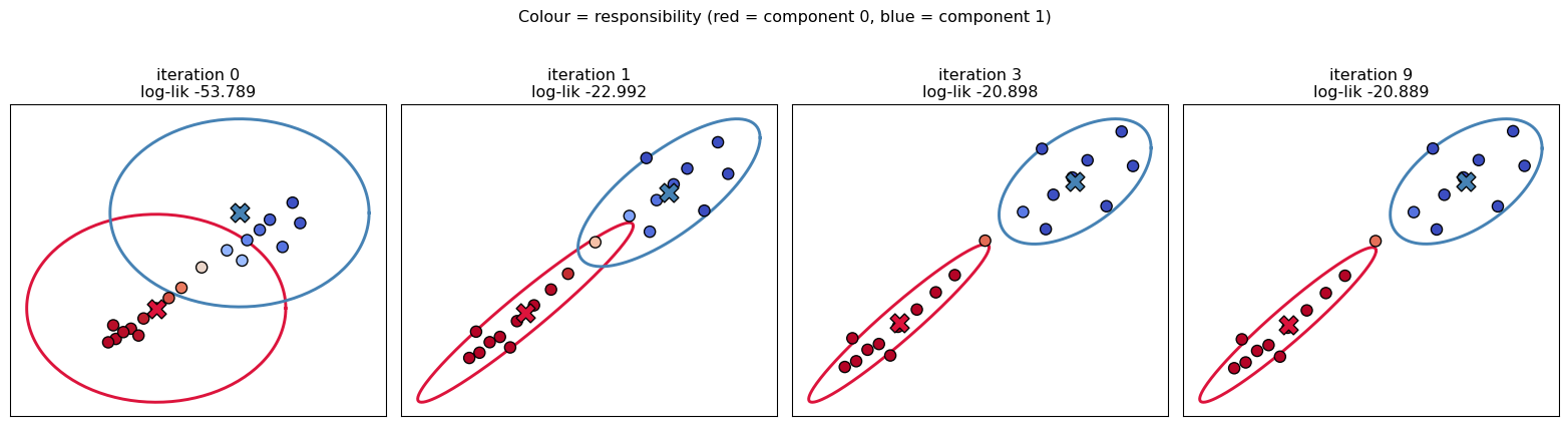
initial means (two random epochs): ['ep05', 'ep15']

   mu_0 = [-0.6319 -0.6343]   pi_0 = 0.5000
   mu_1 = [0.6553 1.3955]   pi_1 = 0.5000

initial log-likelihood: -53.789152

E-STEP, iteration 1 - responsibilities

    id        pi0*N0        pi1*N1           sum    gamma_0    gamma_1   confident?
--------------------------------------------------------------------------------
  ep00  5.293937e-02  3.509963e-04  5.329037e-02   0.993414   0.006586          yes
  ep01  6.709194e-02  9.348445e-04  6.802679e-02   0.986258   0.013742          yes
  ep02  4.649505e-02  2.288812e-04  4.672393e-02   0.995101   0.004899          yes
  ep03  7.625357e-02  2.123583e-03  7.837715e-02   0.972906   0.027094          yes
  ep04  6.152321e-02  6.364842e-04  6.215969e-02   0.989760   0.010240          yes
  ep05  7.957747e-02  4.429342e-03  8.400681e-02   0.947274   0.052726          yes
  ep06  5.981096e-02  6.793876e-04  6.049034e-02   0.988769   0.011231          yes
  ep07  6.479889e-02  7.820655e-04  6.558096e-02   0.988075   0.011925          yes
  ep08  7.625357e-02  8.482997e-03  8.473657e-02   0.899890   0.100110            -
  ep09  4.260103e-02  3.422305e-02  7.682408e-02   0.554527   0.445473   borderline
  ep10  1.037894e-02  6.680099e-02  7.717992e-02   0.134477   0.865523            -
  ep11  2.886328e-03  7.057493e-02  7.346125e-02   0.039290   0.960710          yes
  ep12  2.051053e-02  5.681343e-02  7.732396e-02   0.265255   0.734745            -
  ep13  6.930205e-04  5.556752e-02  5.626054e-02   0.012318   0.987682          yes
  ep14  5.517558e-03  7.097687e-02  7.649442e-02   0.072130   0.927870          yes
  ep15  4.429342e-03  7.957747e-02  8.400681e-02   0.052726   0.947274          yes
  ep16  5.071075e-03  4.911275e-02  5.418382e-02   0.093590   0.906410          yes
  ep17  1.973340e-02  4.751095e-02  6.724434e-02   0.293458   0.706542            -
  ep18  6.709194e-02  1.491762e-02  8.200956e-02   0.818099   0.181901            -
  ep19  1.300638e-03  5.014405e-02  5.144469e-02   0.025282   0.974718          yes
--------------------------------------------------------------------------------

every row sums to 1: True

worked example, the most uncertain epoch (ep09):
   pi_0 * N(x | mu_0, S_0) = 0.5000 * 8.520206e-02 = 4.260103e-02
   pi_1 * N(x | mu_1, S_1) = 0.5000 * 6.844611e-02 = 3.422305e-02
   gamma_0 = 4.260103e-02 / (4.260103e-02 + 3.422305e-02) = 0.554527
   from the array: 0.554527   MATCH: True

   k-means would force this epoch entirely into one cluster. EM records
   that it is 55%/45% - and that uncertainty feeds
   into the M-step.
M-STEP, iteration 1

effective counts N_k = sum of responsibilities:
   N_0 = 0.993 + 0.986 + 0.995 + 0.973 + 0.990 + ... = 11.122599
   N_1 = 0.007 + 0.014 + 0.005 + 0.027 + 0.010 + ... = 8.877401
   N_0 + N_1 = 20.000000  (= n = 20): True

component 0:
   pi_0 = N_0/n = 11.1226/20 = 0.556130
   mu_0 = (weighted sum) / N_0
        = [-8.119  -8.1484] / 11.1226 = [-0.73   -0.7326]
        was [-0.6319 -0.6343]
   Sigma_0 =
       (2, 2) =
            0 |  +0.38074   +0.36765
            1 |  +0.36765   +0.38254

component 1:
   pi_1 = N_1/n = 8.8774/20 = 0.443870
   mu_1 = (weighted sum) / N_1
        = [8.119  8.1484] / 8.8774 = [0.9146 0.9179]
        was [0.6553 1.3955]
   Sigma_1 =
       (2, 2) =
            0 |  +0.27184   +0.19744
            1 |  +0.19744   +0.25870

log-likelihood: -53.789152  ->  -22.991568   (UP by 30.797584)

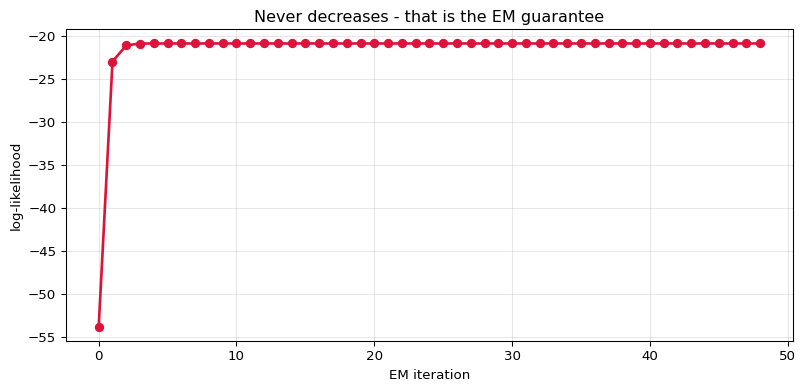
EM guarantees this never decreases - which is the theorem that makes
the algorithm work. It is verified over many iterations below.
Running to convergence
Like k-means, EM is guaranteed to improve its objective every iteration — here the log-likelihood — and therefore to converge. And like k-means, only to a local optimum.
iter     log-likelihood         change   increased?
----------------------------------------------------
    0       -53.78915164                           -
    1       -22.99156800  +30.797583644         True
    2       -21.10820504   +1.883362958         True
    3       -20.89792384   +0.210281203         True
    4       -20.89006748   +0.007856353         True
    5       -20.88948251   +0.000584970         True
    6       -20.88926091   +0.000221601         True
    7       -20.88914680   +0.000114110         True
    8       -20.88908670   +0.000060107         True
    9       -20.88905484   +0.000031854         True
   10       -20.88903790   +0.000016946         True
   11       -20.88902886   +0.000009039         True
   12       -20.88902403   +0.000004829         True
   13       -20.88902145   +0.000002582         True
  ...
   48       -20.88901850
----------------------------------------------------

monotonically non-decreasing throughout? True
converged after 48 iterations


final fit

component 0:  pi = 0.546247,  mu = [-0.826  -0.8162]
   Sigma_0 (2, 2) =
            0 |  +0.20187   +0.20841
            1 |  +0.20841   +0.23457
   eigenvalues [0.0092 0.4273]  -> elongated, axis ratio 6.83

component 1:  pi = 0.453753,  mu = [0.9944 0.9826]
   Sigma_1 (2, 2) =
            0 |  +0.15072   +0.08078
            1 |  +0.08078   +0.15398
   eigenvalues [0.0716 0.2331]  -> elongated, axis ratio 1.81

epochs the model is NOT confident about (max gamma < 0.9):
   ep09: gamma = [0.8358 0.1642]  (true class 0)

That list is information k-means cannot produce at all.
4. K-Means Is a Special Case
Take a Gaussian mixture and impose three restrictions:
- all covariances equal and spherical, $\Sigma_k = \sigma^2 I$
- all mixing weights equal, $\pi_k = 1/K$
- let $\sigma^2 \to 0$
Then the responsibility of the nearest component tends to 1 and every other to 0 — the soft assignment becomes hard, and the M-step reduces to "average the points assigned to me". That is Lloyd's algorithm exactly.
So k-means is not a different method. It is a Gaussian mixture with the covariance thrown away and the uncertainty rounded off, and the demonstration below is just watching $\sigma$ shrink.
a probe point at [0.25 0.  ], between two centres at [-1.  0.] and [1. 0.]

   Euclidean distance to mu_a: 1.2500
   Euclidean distance to mu_b: 0.7500
   -> k-means would assign it to component b, with no hesitation

     sigma         gamma_a         gamma_b                   behaviour
----------------------------------------------------------------------
      2.00    0.4687906266    0.5312093734    almost 50/50 - very soft
      1.00    0.3775406688    0.6224593312                     leaning
      0.50    0.1192029220    0.8807970780                 nearly hard
      0.30    0.0038510324    0.9961489676          HARD, like k-means
      0.20    0.0000037266    0.9999962734          HARD, like k-means
      0.10    0.0000000000    1.0000000000          HARD, like k-means
      0.05    0.0000000000    1.0000000000          HARD, like k-means
      0.01    0.0000000000    1.0000000000          HARD, like k-means
----------------------------------------------------------------------

As sigma shrinks the responsibilities collapse to 0 and 1. In the limit
EM performs exactly the assign-and-average steps of Lloyd's algorithm.


on our 20 epochs

                      method    agreement with k-means
--------------------------------------------------------
   GMM, spherical covariance                   100.0%
        GMM, full covariance                   100.0%
--------------------------------------------------------

With spherical covariances the GMM reproduces k-means almost exactly,
as the theory says. With full covariances it is free to disagree.
The shapes k-means could not find
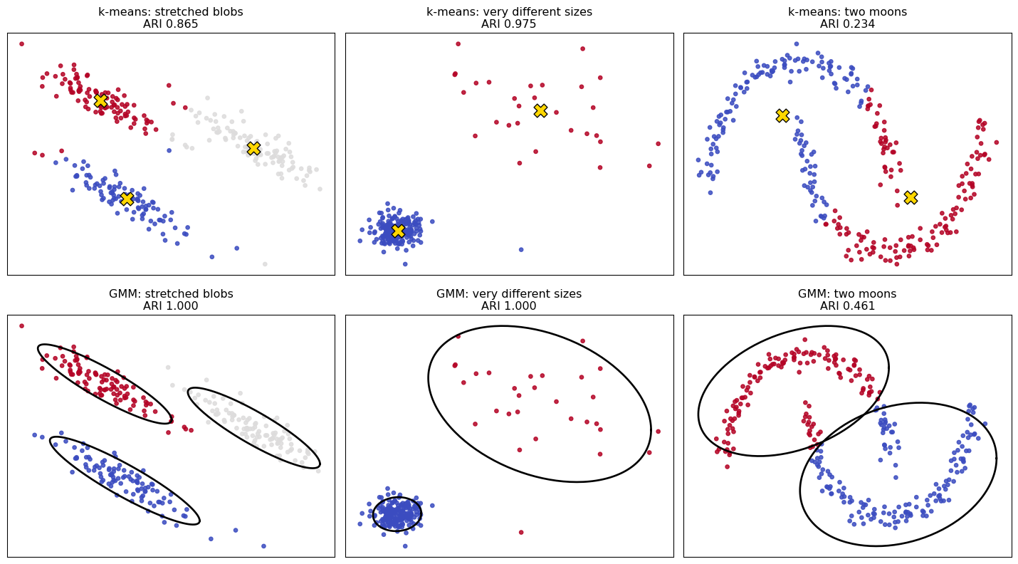
The K-Means walkthrough showed three failure cases. Two of them — stretched clusters and clusters of very different sizes — are caused precisely by the missing covariance and the equal mixing weights. A full-covariance GMM handles both.
The third, the two moons, defeats it too: a mixture of Gaussians is still a mixture of convex blobs, and a crescent is not one. Knowing which failures a richer model fixes, and which it does not, is the useful part.
dataset    k-means ARI    GMM (full) ARI                 verdict
------------------------------------------------------------------------------
       stretched blobs         0.8650            1.0000           GMM solves it
  very different sizes         0.9750            1.0000           GMM solves it
             two moons         0.2343            0.4606  GMM better, still poor
------------------------------------------------------------------------------
Rows: k-means on top, GMM below. The ellipses show what the covariance
bought - they tilt and stretch to match the data.

Read the three rows separately - they are not the same story:
   stretched blobs      - the covariance fixes it outright (ARI 1.00)
   very different sizes - the mixing weights fix this one too
   two moons            - GMM beats k-means, but 0.46 is still poor.
                          It is NOT solved. Every component is an
                          ellipse and no ellipse is a crescent; GMM
                          merely places its ellipses less badly.

For crescents, rings and manifolds the right tools are density-based
(DBSCAN) or spectral methods - not a richer parametric blob.
5. Choosing $K$ — Now There Is a Principled Way
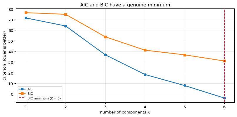
Because a GMM is a probabilistic model, it assigns a likelihood to the data, and that allows information criteria that trade fit against complexity:
$$\text{AIC} = 2p - 2\ln\hat{L} \qquad\qquad \text{BIC} = p\ln n - 2\ln\hat{L}$$
with $p$ the number of free parameters. Both penalise complexity; BIC penalises harder as $n$ grows, so it tends to choose fewer components.
K-means has no such option: its inertia falls monotonically with $K$ and cannot be compared across models. That is a real advantage of the probabilistic formulation, not a detail.
K   params    log-likelihood         AIC         BIC   k-means inertia
--------------------------------------------------------------------------
   1        5          -30.7673     71.5345     76.5132           40.0000
   2       11          -21.0083     64.0166     74.9697            6.5191
   3       17           -1.4456     36.8911     53.8186            3.6837
   4       23           13.8214     18.3572     41.2590            2.2182
   5       29           25.0156      7.9687     36.8449            1.6162
   6       35           36.8864     -3.7727     31.0779            1.3230
--------------------------------------------------------------------------

best by AIC: K = 6
best by BIC: K = 6

k-means inertia just keeps falling - it cannot pick K by itself.
6. Checking Against scikit-learn
log-likelihood (total)
   ours    : -20.8890185000
   sklearn : -20.8890185000
   MATCH: True

means (sorted, since component numbering is arbitrary)

   ours [-0.826  -0.8162]   sklearn [-0.826  -0.8162]
   ours [0.9944 0.9826]   sklearn [0.9944 0.9826]
   MATCH: True

weights

   ours    : [0.5462 0.4538]
   sklearn : [0.5462 0.4538]
   MATCH: True

covariances

   ours:
       (2, 2) =
            0 |  +0.2018692   +0.2084080
            1 |  +0.2084080   +0.2345665
   sklearn:
       (2, 2) =
            0 |  +0.2018693   +0.2084081
            1 |  +0.2084081   +0.2345666

   ours:
       (2, 2) =
            0 |  +0.1507188   +0.0807771
            1 |  +0.0807771   +0.1539773
   sklearn:
       (2, 2) =
            0 |  +0.1507188   +0.0807771
            1 |  +0.0807771   +0.1539772

   MATCH: True

responsibilities MATCH: True
hard assignments MATCH : True


against the withheld true labels
   GMM adjusted Rand index     : 0.7996
   k-means adjusted Rand index : 0.6200
7. Summary
| K-Means | Gaussian Mixture | |
|---|---|---|
| Cluster is | a point | a distribution |
| Assignment | hard, $\{0,1\}$ | soft, $\gamma_{ik}\in[0,1]$ |
| Shape | spherical only | any ellipse, per component |
| Sizes | implicitly equal | $\pi_k$ per component |
| Objective | inertia | log-likelihood |
| Choosing $K$ | elbow / silhouette | AIC / BIC |
| Parameters ($K$=2, $D$=2) | 4 | 11 |
| Cost per iteration | $O(nKD)$ | $O(nKD^2)$ + inverses |
The one idea: EM is Lloyd's algorithm with the hard assignment replaced by a probability. Both alternate "assign, then refit"; only the strength of the assignment differs, and letting it be fractional is what admits covariance, unequal sizes, and a statement of confidence.
The cost of the extra power: more parameters to estimate, so more data needed, plus a
genuine failure mode — a component can collapse onto a single point, driving
$\lvert\Sigma\rvert \to 0$ and the likelihood to infinity. That is why reg_covar exists:
it adds a small constant to the diagonal to stop it.
What it still cannot do: every component is convex. On the two-moons data above GMM scores better than k-means (0.46 vs 0.23) but still fails - no ellipse is a crescent. The extra flexibility buys shape and orientation, not topology.
What is deliberately left out: the proof that EM never decreases the likelihood (via Jensen's inequality and the ELBO), the connection to variational inference, Dirichlet process mixtures that infer $K$, and the tied/diagonal covariance variants that sit between spherical and full.