🧭 How Models Learn: The Concepts
You call .fit(). A second later something is trained. What happened in that second?
Every other walkthrough in this series opens one specific algorithm. This one opens the thing they all share: the idea of learning from data. It is the notebook to read first, and the one to come back to, because every term used elsewhere — loss, gradient, learning rate, bias, variance, overfitting, regularisation — is defined here with numbers you can check on paper.
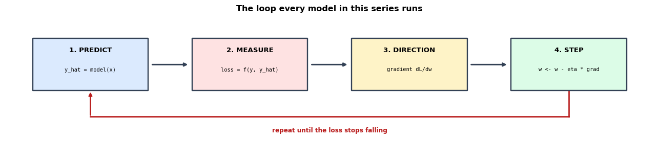
The claim being unpacked is this: training is not magic and it is not search over programs. It is a loop of four steps repeated until the numbers stop improving.
guess → measure how wrong → work out which way is less wrong → move a little → repeat
Everything below is that sentence, made arithmetic. The datasets are tiny on purpose: small enough that every quantity is printed in full, so nothing has to be taken on faith.
Display helpers ready: banner, step, check, expand, show_matrix, show_matmul, show_elementwise.
Flow diagram helper ready: draw_flow(steps, title, loop_label).
1. What a Model Actually Is
Before learning can be discussed, it is worth being precise about what is being learned.
A model is two things:
- A family of functions, fixed in advance by you.
LinearRegressionsays "my answer will have the form $w_0 + w_1x$". A decision tree says "my answer will be a series of threshold questions". Nothing outside the family can ever be produced, no matter how much data arrives. - Parameters, the dials that pick one member out of that family.
So "training" is not the model inventing anything. The shape of the answer was chosen by you when you picked the algorithm. Training only turns the dials.
$$\underbrace{\hat{y} = w_0 + w_1 x}_{\text{the family: chosen by you}} \qquad \underbrace{w_0 = 1.4,\; w_1 = 0.8}_{\text{the parameters: found by training}}$$
This is why "which algorithm should I use?" matters so much: it is the question of which shapes of answer are even reachable.
the data - 8 points, and that is the whole training set

  id       x        y
----------------------
  p0     1.0      2.1
  p1     2.0      3.9
  p2     3.0      6.2
  p3     4.0      7.8
  p4     5.0     10.1
  p5     6.0     12.2
  p6     7.0     13.8
  p7     8.0     16.1
----------------------

three DIFFERENT families of function, each with its own parameters:

   straight line   y = w0 + w1*x                    2 parameters
   parabola        y = w0 + w1*x + w2*x^2           3 parameters
   constant        y = w0                           1 parameter

what each family can produce, using some arbitrary parameter values:

    x   line (1+2x)    parabola (1+2x-0.1x^2)   constant (9)
------------------------------------------------------------
  1.0          3.00                      2.90           9.00
  2.0          5.00                      4.60           9.00
  3.0          7.00                      6.10           9.00
  4.0          9.00                      7.40           9.00
------------------------------------------------------------

The constant family can NEVER produce a sloped answer - not with any
parameter value, not with any amount of data. That is a limit of the
family, not of the training. Choosing the algorithm chooses the limits.
2. The Loss — Turning "Wrong" Into a Number
Learning needs a target to improve. That means "how wrong is this model?" has to become a single number, because you cannot minimise a feeling.
$$\text{loss} = \text{one number summarising all the errors}$$
Start with the per-point error, then decide how to combine them. The choice of how is not cosmetic — it changes what the model ends up believing.
a guess: w0 = 0.5, w1 = 1.8

  id      x        y          prediction      error   |error|    error^2
----------------------------------------------------------------------
  p0    1.0      2.1  0.5 + 1.8*1 =   2.30     -0.200     0.200     0.0400
  p1    2.0      3.9  0.5 + 1.8*2 =   4.10     -0.200     0.200     0.0400
  p2    3.0      6.2  0.5 + 1.8*3 =   5.90      0.300     0.300     0.0900
  p3    4.0      7.8  0.5 + 1.8*4 =   7.70      0.100     0.100     0.0100
  p4    5.0     10.1  0.5 + 1.8*5 =   9.50      0.600     0.600     0.3600
  p5    6.0     12.2  0.5 + 1.8*6 =  11.30      0.900     0.900     0.8100
  p6    7.0     13.8  0.5 + 1.8*7 =  13.10      0.700     0.700     0.4900
  p7    8.0     16.1  0.5 + 1.8*8 =  14.90      1.200     1.200     1.4400
----------------------------------------------------------------------
                                     SUM      3.400     4.200     3.2800

three ways to make one number out of that column:

   sum of errors        = +3.4000   <- USELESS: +3 and -3 cancel
   mean absolute error  = 4.2000 / 8 = 0.5250
   mean squared error   = 3.2800 / 8 = 0.4100

The first is discarded immediately: a model that is +10 on one point and
-10 on another would score a perfect 0. Errors must be made positive
first, either by |.| or by squaring.
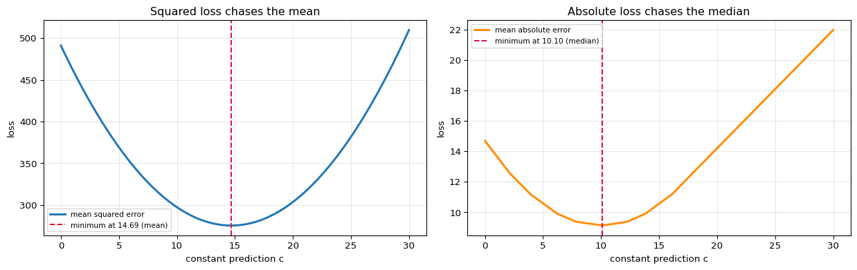
Squaring vs absolute value is a real decision
They are not two spellings of the same thing. Squaring makes a big error count disproportionately: an error of 4 costs 16, while four errors of 1 cost 4 in total. So squared loss will contort the model to avoid one large mistake.
The consequence is provable and worth knowing:
$$\text{minimising } \sum(y_i - c)^2 \;\Rightarrow\; c = \text{mean}(y) \qquad\qquad \text{minimising } \sum|y_i - c| \;\Rightarrow\; c = \text{median}(y)$$
The loss you pick decides what "typical" means to your model. That is why squared loss is sensitive to outliers and absolute loss is not.
data plus one outlier: [2.1, 3.9, 6.2, 7.8, 10.1, 12.2, 13.8, 16.1, 60.0]

searching every constant c from 0 to 30 for the one that minimises each loss:

      c    mean squared    mean absolute
----------------------------------------
    8.0        320.0222           9.3556
   10.0        297.2667           9.1333
   12.0        282.5111           9.3333
   14.0        275.7556          10.0000
   16.0        277.0000          11.1111
   18.0        286.2444          12.6444
----------------------------------------

best c under squared loss  : 14.6900
mean of the data           : 14.6889   MATCH: True

best c under absolute loss : 10.1000
median of the data         : 10.1000   MATCH: True

The single outlier at 60 dragged the squared-loss answer to 14.69,
while the absolute-loss answer stayed at 10.10, near the bulk of
the data. Same data, same 'best' - two different definitions of best.
Note the shapes: squared loss is a smooth bowl (differentiable everywhere),
absolute loss has a kink at the minimum. That kink is exactly why squared
loss is the default - it is easier to optimise, as the next section shows.
3. The Learning Loop
With a loss defined, learning becomes a concrete question: which parameter values make this number small?
For a two-parameter model you could try every combination. For a neural network with a million parameters you obviously cannot. So instead of searching, learning uses a local rule: from wherever you are, work out which direction is downhill, and step that way.
What changes between algorithms is only the CONTENTS of the boxes:

             algorithm              box 1: predict             box 2: loss
--------------------------------------------------------------------------
     Linear regression                   w0 + w1*x           squared error
   Logistic regression                sigmoid(w.x)                log-loss
        Neural network        layers + activations          log-loss / MSE
                   SVM               sign(w.x + b)         hinge + ||w||^2
               XGBoost                sum of trees        any, via g and h
--------------------------------------------------------------------------

The loop itself never changes. Decision trees and k-means are the
exceptions in this series - they minimise their objective by a different
device (greedy splitting, alternating assignment) - but even there the
skeleton is the same: measure, improve, repeat.
4. The Gradient — Which Way Is Downhill
Box 3 is where the actual mathematics lives, and it is one idea: the derivative tells you how the loss responds to a nudge.
$$\frac{\partial \mathcal{L}}{\partial w} \;\approx\; \frac{\mathcal{L}(w + \epsilon) - \mathcal{L}(w - \epsilon)}{2\epsilon}$$
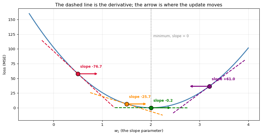
Read it as a rate of exchange: if I increase $w$ by one unit, the loss changes by this much. Three cases, and the rule follows from them:
| Derivative | Meaning | What to do |
|---|---|---|
| positive | increasing $w$ makes things worse | decrease $w$ |
| negative | increasing $w$ makes things better | increase $w$ |
| zero | flat — a nudge either way changes nothing | stop |
All three cases are "move opposite the derivative", which is why the update is $w \leftarrow w - \eta\,\partial\mathcal{L}/\partial w$ — the minus sign is the whole algorithm.
hold w0 = 0 and vary only the slope w1, so the loss is a curve we can walk

     w1         loss    numerical derivative                       reading
--------------------------------------------------------------------------
   0.00    102.42500             -102.200000         downhill to the RIGHT
   0.50     57.70000              -76.700000         downhill to the RIGHT
   1.00     25.72500              -51.200000         downhill to the RIGHT
   1.50      6.50000              -25.700000         downhill to the RIGHT
   1.90      0.30000               -5.300000         downhill to the RIGHT
   2.00      0.02500               -0.200000         downhill to the RIGHT
   2.50      6.30000               25.300000          downhill to the LEFT
   3.00     25.32500               50.800000          downhill to the LEFT
--------------------------------------------------------------------------

one derivative worked out fully, at w1 = 1.0:

   loss at w1 = 1.00001  ->  25.7244880025
   loss at w1 = 0.99999  ->  25.7255120026
   change in loss          = -0.0010240000
   change in w1            = 0.0000200000
   ratio (the derivative)  = -51.200000

   the same thing from calculus, dL/dw1 = (2/n) * sum((w1*x - y)*x):
      = (2/8) * (-1.10 + -3.80 + -9.60 + -15.20 + -25.50 + ...)
      = (2/8) * -204.800000 = -51.200000
   numerical: -51.200000   MATCH: True

   Negative, so the loss falls if w1 increases - and indeed the bottom
   of the curve is further right, near w1 = 2.
Every arrow points toward the bottom, and every arrow points OPPOSITE its
dashed tangent line. That is the minus sign doing its job.

At the minimum (w1 = 2.004) the tangent is horizontal - the
derivative is zero, no direction improves anything, and learning stops.
'Converged' means exactly this and nothing more.
5. The Learning Rate — How Big a Step
The gradient gives a direction but not a distance. The learning rate $\eta$ supplies the distance, and it is the single most consequential number you set by hand.
$$w \leftarrow w - \eta\,\frac{\partial\mathcal{L}}{\partial w}$$
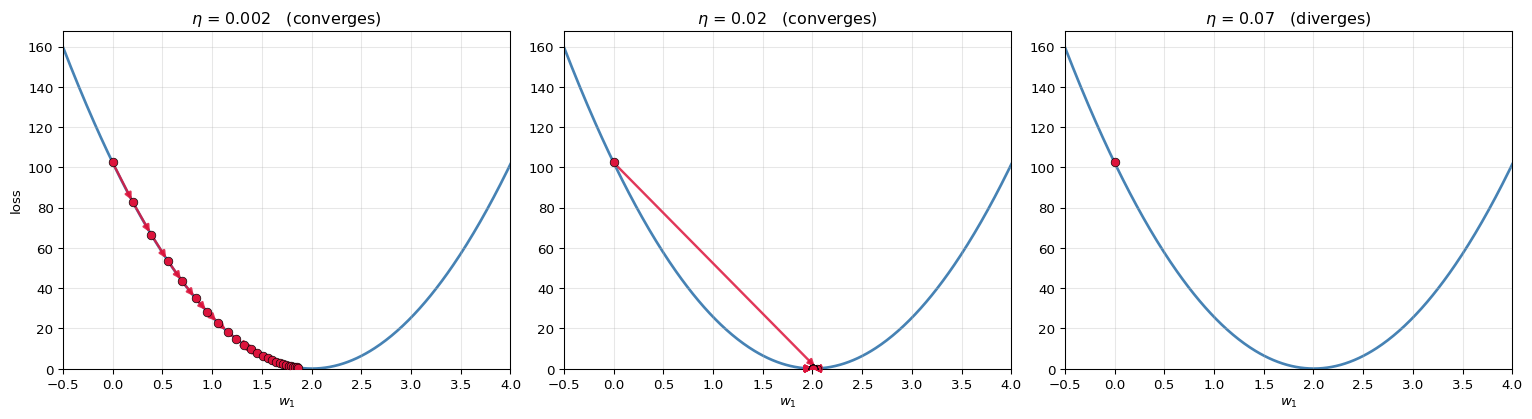
Three regimes, all visible below:
- $\eta$ too small — correct every step, but arrives too slowly to be useful
- $\eta$ about right — steady approach, steps shortening naturally as the gradient shrinks
- $\eta$ too large — each step jumps past the minimum onto the opposite wall, where the gradient is larger still, so the next jump is worse. The loss increases and the model diverges.
Note the third case carefully: nothing is wrong with the direction. It is right every single time. Only the step length is wrong.
the first six steps at three learning rates, starting from w1 = 0

eta = 0.002
   step 0: w1 =    0.0000   loss =   102.4250   grad =  -102.2000   ->  w1 = 0.0000 - 0.002*(-102.2000) =    0.2044
   step 1: w1 =    0.2044   loss =    82.6007   grad =   -91.7756   ->  w1 = 0.2044 - 0.002*(-91.7756) =    0.3880
   step 2: w1 =    0.3880   loss =    66.6143   grad =   -82.4145   ->  w1 = 0.3880 - 0.002*(-82.4145) =    0.5528
   step 3: w1 =    0.5528   loss =    53.7228   grad =   -74.0082   ->  w1 = 0.5528 - 0.002*(-74.0082) =    0.7008
   step 4: w1 =    0.7008   loss =    43.3270   grad =   -66.4594   ->  w1 = 0.7008 - 0.002*(-66.4594) =    0.8337
   step 5: w1 =    0.8337   loss =    34.9439   grad =   -59.6805   ->  w1 = 0.8337 - 0.002*(-59.6805) =    0.9531

eta = 0.02
   step 0: w1 =    0.0000   loss =   102.4250   grad =  -102.2000   ->  w1 = 0.0000 - 0.02*(-102.2000) =    2.0440
   step 1: w1 =    2.0440   loss =     0.0656   grad =     2.0440   ->  w1 = 2.0440 - 0.02*(2.0440) =    2.0031
   step 2: w1 =    2.0031   loss =     0.0246   grad =    -0.0409   ->  w1 = 2.0031 - 0.02*(-0.0409) =    2.0039
   step 3: w1 =    2.0039   loss =     0.0246   grad =     0.0008   ->  w1 = 2.0039 - 0.02*(0.0008) =    2.0039
   step 4: w1 =    2.0039   loss =     0.0246   grad =    -0.0000   ->  w1 = 2.0039 - 0.02*(-0.0000) =    2.0039
   step 5: w1 =    2.0039   loss =     0.0246   grad =     0.0000   ->  w1 = 2.0039 - 0.02*(0.0000) =    2.0039

eta = 0.07
   step 0: w1 =    0.0000   loss =   102.4250   grad =  -102.2000   ->  w1 = 0.0000 - 0.07*(-102.2000) =    7.1540
   step 1: w1 =    7.1540   loss =   676.3690   grad =   262.6540   ->  w1 = 7.1540 - 0.07*(262.6540) =  -11.2318
   step 2: w1 =  -11.2318   loss =  4467.2114   grad =  -675.0208   ->  w1 = -11.2318 - 0.07*(-675.0208) =   36.0197
   step 3: w1 =   36.0197   loss = 29505.3467   grad =  1734.8034   ->  w1 = 36.0197 - 0.07*(1734.8034) =  -85.4166
   step 4: w1 =  -85.4166   loss = 194879.7266   grad = -4458.4448   ->  w1 = -85.4166 - 0.07*(-4458.4448) =  226.6746
   step 5: w1 =  226.6746   loss = 1287160.9709   grad = 11458.2030   ->  w1 = 226.6746 - 0.07*(11458.2030) = -575.3996

the stability limit, from the curvature of the loss:
   d2L/dw1^2 = (2/n) * sum(x^2) = 51.000000
   gradient descent is stable while eta < 2 / 51.000000 = 0.039216

   eta = 0.002  ->  0.05x the limit  : converges, slowly
   eta = 0.020  ->  0.51x the limit  : converges well
   eta = 0.070  ->  1.79x the limit  : DIVERGES
Left  : tiny steps, still far from the bottom after 25 of them.
Middle: steps shorten by themselves as the slope flattens - no tuning needed.
Right : each step overshoots to a HIGHER point on the far wall, so the
        next gradient is larger and the next jump bigger still.
6. Where Error Comes From: Bias, Variance, Noise
Now the concepts that decide whether a trained model is any good.
Suppose there is a true relationship $f(x)$, and what we observe is that plus unpredictable noise:
$$y = f(x) + \varepsilon, \qquad \varepsilon \sim \mathcal{N}(0, \sigma^2)$$
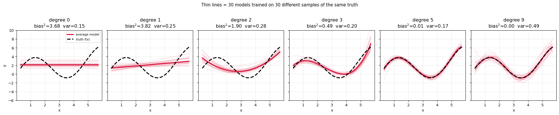
Train on one dataset and you get one model. Train on a different sample from the same source and you get a slightly different model. Repeating that, the expected squared error at a point splits into exactly three parts:
$$\underbrace{\mathbb{E}\big[(y - \hat{f}(x))^2\big]}_{\text{total error}} = \underbrace{\big(\mathbb{E}[\hat{f}(x)] - f(x)\big)^2}_{\textbf{bias}^2} + \underbrace{\mathbb{E}\big[(\hat{f}(x) - \mathbb{E}[\hat{f}(x)])^2\big]}_{\textbf{variance}} + \underbrace{\sigma^2}_{\textbf{noise}}$$
In words, and this is the part worth memorising:
- Bias — how far the average model is from the truth. High bias = the family is too simple to represent $f$. It is wrong consistently.
- Variance — how much the model changes when the training data changes. High variance = it is chasing the particular noise in this sample. It is wrong inconsistently.
- Noise — the part nobody can ever predict. An error floor, not a fault of the model.
Below, all three are computed numerically from a known truth — and their sum is checked against the measured total error.
the experiment: draw 400 independent training sets of 40 points
from the SAME truth, fit a model to each, and see how the predictions
scatter around the true function.

   true f(x)   = 3*sin(1.3x) + 0.6x       (known to us, not to the model)
   noise sigma = 1.0  ->  irreducible error sigma^2 = 1.0

 degree       bias^2     variance      noise   sum = expected err               character
------------------------------------------------------------------------------------------
      0       3.6794       0.1466     1.0000               4.8261          far too simple
      1       3.8182       0.2495     1.0000               5.0676          far too simple
      2       1.8991       0.2777     1.0000               3.1769        still too simple
      3       0.4881       0.2008     1.0000               1.6889                  closer
      5       0.0084       0.1722     1.0000               1.1806             about right
      9       0.0010       0.4860     1.0000               1.4869            too flexible
------------------------------------------------------------------------------------------

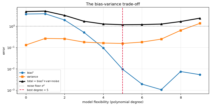
Read the two middle columns as a see-saw: as the model gets more flexible,
bias falls and variance rises. Degree 5 is where their SUM is smallest -
and that sum, not either column alone, is what we actually care about.
Verifying the decomposition
The formula claims $\text{bias}^2 + \text{variance} + \sigma^2$ equals the expected squared error on fresh data. That is a testable claim, not a definition — so it is tested: measure the actual error on newly generated test points and compare.
measuring the true expected error directly, on fresh noisy test data

 degree   measured error   bias^2 + var + noise    difference    match
----------------------------------------------------------------------
      0           4.8120                 4.8261       -0.0140     True
      1           5.0422                 5.0676       -0.0254     True
      2           3.1854                 3.1769       +0.0086     True
      3           1.6852                 1.6889       -0.0037     True
      5           1.1836                 1.1806       +0.0030     True
      9           1.4861                 1.4869       -0.0008     True
----------------------------------------------------------------------

The three parts add up to the error we actually observe. The
decomposition is not a metaphor - it is an identity, and these are the
numbers that confirm it.


what the individual fits look like at one x, say x = 3.0:

   true value f(3.0) = -0.2327

 degree   mean prediction       bias   spread (sd)                   5 individual fits
--------------------------------------------------------------------------------------
      0            2.1476    +2.3803        0.3829   +2.24   +2.45   +2.44   +2.28   +1.83
      1            2.1262    +2.3589        0.3605   +2.12   +2.65   +2.52   +2.26   +2.72
      2            0.6241    +0.8568        0.4557   +0.41   +0.51   +0.94   +0.92   +0.26
      3            0.6687    +0.9014        0.3315   +0.72   +0.74   +0.73   +0.84   +0.53
      5           -0.1265    +0.1062        0.3289   +0.00   -0.26   -0.31   -0.51   +0.15
      9           -0.2780    -0.0453        0.4676   -0.65   +0.96   -0.55   -0.35   -0.24
--------------------------------------------------------------------------------------

Degree 0: every fit lands near the same wrong place - consistent, biased.
Degree 12: the fits are scattered wildly - each one chased its own noise.
degree      bias^2    variance       total
------------------------------------------
      0      3.6836      0.1304      4.8141
      1      3.8009      0.2643      5.0652
      2      1.9329      0.2569      3.1898
      3      0.5113      0.1779      1.6892
      4      0.0956      0.1612      1.2568
      5      0.0095      0.1540      1.1636  <== best
      6      0.0019      0.1784      1.1803
      7      0.0011      0.2461      1.2472
      8      0.0074      0.6319      1.6394
      9      0.0053      1.3524      2.3577
------------------------------------------

The total can never go below the noise floor of 1.00. Chasing
error below that is chasing randomness, and it is exactly what
overfitting is.
7. Underfitting and Overfitting
Those two failure modes have names, and now they have precise meanings:
| Bias | Variance | Train error | Test error | |
|---|---|---|---|---|
| Underfitting | high | low | high | high |
| Good fit | low | low | low | low |
| Overfitting | low | high | very low | high |
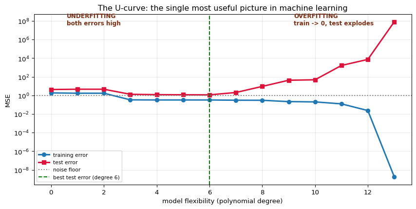
The diagnostic is the gap:
- Train error high and test error high → underfitting. The model is too simple; more data will not help.
- Train error near zero but test error high → overfitting. The model memorised the sample, including its noise.
This is why training error is not a measure of quality. A model can drive it to zero by memorising, which is the opposite of learning.
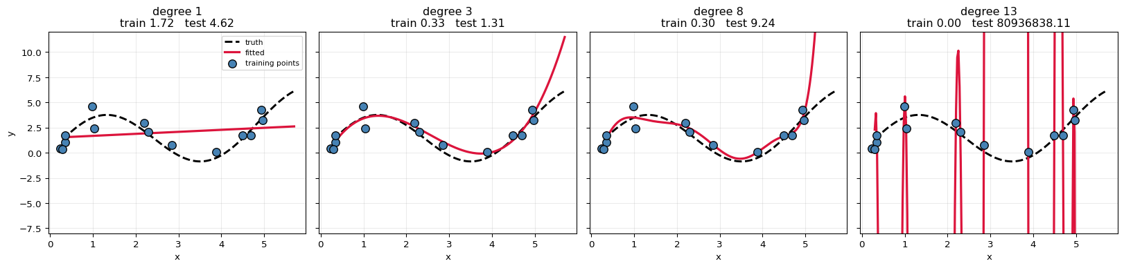
one training set of 14 points, one test set of 400 points

 degree   params    train MSE    test MSE        gap       diagnosis
--------------------------------------------------------------------
      0        1       1.8507      4.2610    +2.4103            good
      1        2       1.7182      4.6218    +2.9036            good
      2        3       1.7180      4.5971    +2.8791            good
      3        4       0.3324      1.3147    +0.9822            good
      4        5       0.3227      1.2020    +0.8793            good
      5        6       0.3225      1.1708    +0.8483            good
      6        7       0.3221      1.1441    +0.8220            good
      7        8       0.3033      2.0471    +1.7438         OVERFIT
      8        9       0.2973      9.2424    +8.9450         OVERFIT
      9       10       0.2144     42.5831   +42.3687         OVERFIT
     10       11       0.1999     47.6812   +47.4814         OVERFIT
     11       12       0.1230   1652.4057  +1652.2828         OVERFIT
     12       13       0.0234   7392.4250  +7392.4015         OVERFIT
     13       14       0.0000  80936838.1121  +80936838.1121         OVERFIT
--------------------------------------------------------------------

lowest TEST error at degree 6
lowest TRAIN error at degree 13  <- train error just keeps falling, and says nothing useful

training points: 14.  At degree 13 the polynomial has as many
free parameters as there are points, so it can pass EXACTLY through every
one of them - train error zero, and a useless model.
Degree 13 passes through every training point perfectly and is wrong
everywhere between them. It has learned the SAMPLE, not the PATTERN.
   train MSE at degree 13: 0.0000000018   <- exactly zero
   test  MSE at degree 13: 80,936,838.1
   noise floor            : 1.00

No ratio is quoted because the training error is exactly 0 - the model
passes through every training point by construction, so 'how many times
worse' is undefined. That is the cleanest statement of the failure:
perfect on data it has seen, useless on data it has not.
8. Why You Must Hold Data Back
The previous section quietly used a test set. That was not a convenience — it is the only way to detect overfitting at all, because from the training data alone the overfitted model looks perfect.
When data is scarce, one split wastes most of it. $k$-fold cross-validation reuses everything: split into $k$ parts, train on $k-1$ and test on the one held out, rotate, and average.
$$\text{CV score} = \frac{1}{k}\sum_{j=1}^{k}\text{error on fold } j$$
Every point is used for training $k-1$ times and for testing exactly once.
7-fold cross-validation on the 14 training points

 fold         test points    train points
------------------------------------------
    0             [1, 10]              12
    1              [7, 9]              12
    2             [4, 13]              12
    3              [5, 8]              12
    4              [0, 2]              12
    5            [11, 12]              12
    6              [3, 6]              12
------------------------------------------

 degree       f0       f1       f2       f3       f4       f5       f6    CV mean   true test
------------------------------------------------------------------------------
      1     4.30     1.28     2.98     1.14     5.37     2.57     0.34      2.567       4.622
      2     4.59     1.34     4.68     1.43     5.52     3.22     0.40      3.024       4.597
      3     0.51     0.66     0.35     1.33     1.37     0.75     0.21      0.739       1.315
      4     0.78     0.59     0.27     2.50     1.79     0.96     0.23      1.017       1.202
      5     0.78     1.04     0.33     2.53     1.99     1.10     0.44      1.173       1.171
      8   200.59     2.66   323.96     5.85     2.50     1.33     1.39     76.899       9.242
     13  4661315721.06  2237334.03  2161.83  1393932.78     2.72    29.89  5300931.99  667178587.758  80936838.112
------------------------------------------------------------------------------

CV picks degree 3; the true test error is lowest at degree 6.
CV chose a different model - and it did so WITHOUT ever touching the test set.

That is the point: cross-validation lets you choose a model using only
training data, keeping the test set genuinely unseen for the final
estimate. Choosing with the test set and then reporting its score is
how people accidentally report numbers they cannot reproduce.
9. Regularisation — Buying Bias to Sell Variance
Section 6 showed the trade-off; regularisation is the dial that moves along it. Add a penalty on parameter size to the loss:
$$\mathcal{L}_{\text{total}} = \underbrace{\sum_i(y_i - \hat{y}_i)^2}_{\text{fit the data}} \;+\; \underbrace{\lambda\sum_j w_j^2}_{\text{stay small}}$$
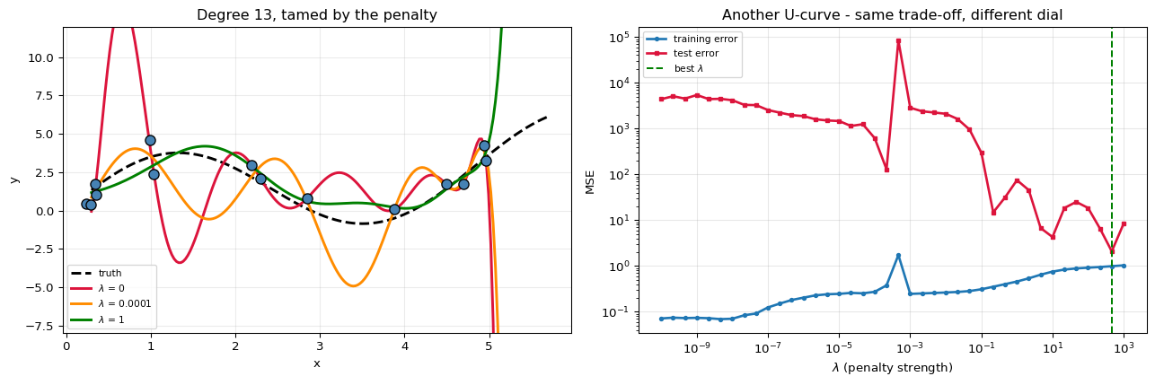
The model now pays for complexity. Wiggly high-degree curves need large coefficients, so the penalty suppresses them — without removing them from the family.
This deliberately increases bias in exchange for a larger reduction in variance. When that trade is favourable, total error falls.
a degree-13 model - the one that overfitted badly - with increasing lambda

    lambda    train MSE    test MSE    max |coef|       sum w^2
--------------------------------------------------------------
     0e+00      0.07082   6264.8707          5166       5.8e+07
     1e-08      0.07025   4152.6497          4032     3.553e+07
     1e-06      0.20301   1869.0047         305.1     2.661e+05
     1e-04      0.27211    618.2217         23.32          1275
     1e-02      0.26296   2102.6247         4.195         27.65
     1e+00      0.45646     74.7813        0.8584         1.588
     1e+02      0.91503     18.4542           1.7      0.006202
--------------------------------------------------------------

best test error at lambda = 1e+02
   with no penalty  : train 0.07082, test 6264.87
   with the penalty : train 0.91503, test 18.45

Train error got WORSE and test error got much better. That exchange is
the entire purpose - and it is why judging a model by training error
would have told you to throw the regularisation away.

Too little penalty: overfitting, as before.
Too much penalty  : the coefficients are crushed to nothing and the model
                    underfits. Regularisation can cause EITHER failure.
10. What More Data Does
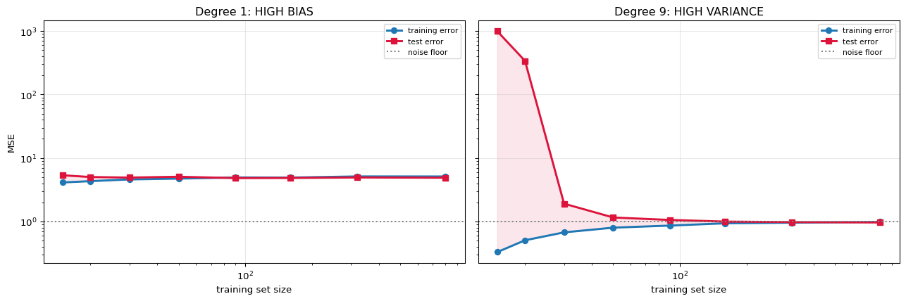
The last lever. A learning curve plots error against training-set size, and it diagnoses which problem you have — which decides whether collecting more data is worth the effort.
- High variance (overfitting) — a large gap between train and test error that narrows as data arrives. More data helps.
- High bias (underfitting) — both curves flatten early, close together, at a poor value. More data does nothing. You need a better model family, not a bigger sample.
This is one of the few pictures that tells you what to do next.
n_train   deg1 train    deg1 test   deg9 train    deg9 test
------------------------------------------------------------
       15        4.112        5.337        0.329      993.042
       20        4.313        5.011        0.505      339.077
       30        4.591        4.911        0.672        1.905
       50        4.730        5.062        0.798        1.153
       90        4.931        4.817        0.860        1.055
      160        4.912        4.843        0.935        0.994
      320        5.120        4.929        0.956        0.976
      800        5.110        4.881        0.985        0.963
------------------------------------------------------------

gap between test and train at n = 800:
   degree 1  : -0.2294   (already closed - and stuck well above the
               noise floor of 1.00, so the model itself is the limit)
   degree 9  : -0.0222   (closing as data arrives)

degree 9 at n= 15: test error   993.04
degree 9 at n=800: test error     0.96   -> data fixed it
degree  1 at n= 15: test error     5.34
degree  1 at n=800: test error     4.88   -> data changed nothing

Same problem, same extra data, opposite conclusions. That is why the
first question after a disappointing model is 'which curve am I on?'
11. Where Each Concept Shows Up
Everything above is deliberately algorithm-free, because it applies to all of them. This table maps each idea onto the specific walkthroughs, so a term met elsewhere can be traced back here.
| Concept | In this notebook | Where it appears in the algorithms |
|---|---|---|
| Loss | section 2 | squared error (Linear Regression), log-loss (Logistic, Neural Net), hinge (SVM), Gini (Decision Tree), inertia (K-Means) |
| Gradient | section 4 | $X^\top(\mathbf{p}-\mathbf{y})$ in Logistic, $\delta$ in backpropagation, $g_i$ in XGBoost |
| Learning rate | section 5 | $\eta$ in Linear/Logistic/Neural Net, eta (shrinkage) in XGBoost and LightGBM |
| Bias / variance | section 6 | why forests average trees; why $k$ matters in KNN; why boosting adds shallow trees |
| Overfitting | section 7 | a single deep Decision Tree; RBF SVM with large $\gamma$; large num_leaves in LightGBM |
| Held-out data | section 8 | OOB error in Random Forest; leave-one-out in KNN |
| Regularisation | section 9 | ridge/lasso in Linear Regression; $C$ in SVM; $\lambda$ and $\gamma$ in XGBoost; ordered boosting in CatBoost |
| Capacity | sections 6–10 | polynomial degree here; tree depth; hidden units; number of components in PCA |
12. Summary
$$\text{total error} \;=\; \underbrace{\text{bias}^2}_{\text{too simple}} \;+\; \underbrace{\text{variance}}_{\text{too sensitive}} \;+\; \underbrace{\sigma^2}_{\text{unavoidable}}$$
Six things worth carrying away:
- Training turns dials, it does not invent shapes. The family of possible answers was fixed when you chose the algorithm.
- The loss defines what "good" means. Change it and you change the model's idea of a typical value — squared loss chases the mean, absolute loss the median.
- The gradient supplies direction; the learning rate supplies distance. A correct direction with too large a step still diverges.
- Error has three parts, and they are measurable. Bias and variance move in opposite directions; the noise floor cannot be crossed by any model.
- Training error is not quality. Any sufficiently flexible model can drive it to zero by memorising, which is why held-out data is not optional.
- The learning curve tells you what to do next. Gap still closing → get more data. Both curves flat and poor → more data will not help; change the model.
What is deliberately left out: momentum and adaptive optimisers (Adam), stochastic gradient noise as implicit regularisation, the double-descent phenomenon in very over-parameterised models, formal generalisation bounds (VC dimension, PAC learning), nested cross-validation, and everything about data quality — leakage, drift, imbalance — which matters enormously in practice and is a separate subject from how learning works.