🔎 Hyperparameter Search
Hyperparameter Search
Hyperparameters are the settings you choose rather than learn — a tree's depth, a ridge penalty, a learning rate. The search for good ones is usually the last thing anyone thinks about and the first thing that wastes a week of compute.
Three strategies, in increasing order of cleverness:
| how it picks the next configuration | when it wins | |
|---|---|---|
| Grid search | every combination on a lattice | few parameters, all of them mattering |
| Random search | independent draws from a distribution | most real problems |
| Bayesian / TPE | fits a model of the objective, optimises an acquisition function | evaluations are expensive |
The interesting result is the middle row. Random search sounds like the lazy option and usually beats grid search — for a reason that is arithmetic, not folklore, and that this page works out in full.
Display helpers ready: banner, step, check, expand, show_matrix, show_matmul, show_elementwise.
==============================================================================
  A SMALL PROBLEM WITH REAL SIGNAL IN IT
==============================================================================
  300 samples, 20 features, 5 informative
  class balance: [150, 150]

Baseline: default SVC, no tuning
==============================================================================
  default SVC  : [0.8333 0.8667 0.8    0.9    0.8333]  mean 0.8467
1. Grid search, written out
A grid is the product of the values you list for each parameter. For an SVC with $C \in \{0.1, 1, 10, 100\}$ and $\gamma \in \{0.001, 0.01, 0.1, 1\}$ that is $4 \times 4 = 16$ configurations, and with 5-fold CV, $16 \times 5 = 80$ model fits.
The cost is the product of everything. Add a third parameter with 4 values and you are at 320 fits; a fourth and you are at 1280. This is the whole problem with grids — they multiply.
==============================================================================
  GRID SEARCH, EVERY CELL SHOWN
==============================================================================

4 x 4 = 16 configurations, 80 fits
==============================================================================
  C  v / gamma >     0.001      0.01       0.1         1
  --------------------------------------------------
         0.1    0.7733    0.8033    0.8167    0.5100
           1    0.7933    0.8300    0.8600    0.6067
          10    0.8100    0.8267    0.8467    0.6000
         100    0.8100    0.7900    0.8467    0.6000
  --------------------------------------------------
  best: C=1, gamma=0.1  ->  0.8600
  (default was 0.8467)

Check against scikit-learn
==============================================================================
  by hand      : C=1, gamma=0.1, 0.860000
  scikit-learn : {'C': 1, 'gamma': 0.1}, 0.860000
  MATCH: True

How the cost multiplies
==============================================================================
   parameters   values each    configs   fits (5-fold)
  ----------------------------------------------------
            1             4          4              20
            2             4         16              80
            3             4         64             320
            4             4        256           1,280
            5             4      1,024           5,120
  ----------------------------------------------------
  Five parameters at four values each is 5,120 fits to explore what is
  still a very coarse lattice -- four values per axis.
2. Why random search beats grid search
This is Bergstra and Bengio's argument (2012), and it is worth working out because the conclusion is counter-intuitive until you see the arithmetic.
The observation: in most problems, not all hyperparameters matter. One or two dominate, the rest barely move the score. But you do not know in advance which.
What a grid does with 25 evaluations. A $5\times5$ grid tests 5 distinct values of each parameter. If only the first parameter matters, you have spent 25 evaluations learning about 5 values of it — the other axis was wasted, five times over.
What random search does with 25 evaluations. Every draw is a fresh value of every parameter. So you test 25 distinct values of the important one — five times the resolution, for identical cost.
The probability statement is exact. If you want a configuration in the top $q$ fraction of the important parameter's range, and you draw $n$ points at random:
$$P(\text{at least one in the top } q) = 1 - (1-q)^n$$
For $q = 0.05$ and $n = 60$: $1 - 0.95^{60} = 0.954$. Sixty random draws give a 95% chance of landing in the best 5% — regardless of how many dimensions you are searching, which is precisely what a grid cannot promise.
==============================================================================
  GRID vs RANDOM: THE RESOLUTION ARGUMENT
==============================================================================

Distinct values tested per parameter, for the same budget
==============================================================================
   budget    grid layout   distinct/param   random: distinct/param
  ----------------------------------------------------------------
        9          3 x 3                3                        9
       16          4 x 4                4                       16
       25          5 x 5                5                       25
       36          6 x 6                6                       36
  ----------------------------------------------------------------
  Same number of model fits. Random tests every value it draws;
  a grid re-tests the same few values over and over.

The probability formula, verified by simulation
==============================================================================
  P(at least one draw in the top q) = 1 - (1-q)^n

       q      n    formula    simulated    MATCH
  ----------------------------------------------
    0.05     20     0.6415       0.6439     True
    0.05     60     0.9539       0.9561     True
    0.10     20     0.8784       0.8789     True
    0.01    100     0.6340       0.6333     True
    0.20     10     0.8926       0.8952     True
  ----------------------------------------------
  Note what is ABSENT from the formula: the number of dimensions.
  60 random draws give a 95% chance of hitting the top 5% of the
  important parameter whether you are searching 2 knobs or 20.

Simulating a problem where only one of five knobs matters
==============================================================================
  budget = 36 evaluations each, 400 repeated trials

  the optimum sits at v[0] = 0.70
  grid lattice on v[0]: [0.05, 0.23, 0.41, 0.59, 0.77, 0.95]
  nearest lattice point: 0.77  -> off by 0.07,
  and no amount of budget on that lattice will close the gap.

  grid   6x6 (mean)         : 0.0085
  random 36 draws (mean)   : 0.0285
  random wins in 87% of trials

  Two things are working for random search here. It is not confined
  to a lattice on v[0], so it can land arbitrarily close to 0.70; and
  it varies v[1..4] too, which the grid pinned at 0.5 -- so it also
  picks up the small contribution from those. Both are the same
  point: the grid spent its budget on a shape chosen in advance.
3. Bayesian optimisation, by hand
Grid and random search are both non-adaptive — every configuration is chosen without reference to what the previous ones scored. When each evaluation is expensive, that is wasteful.
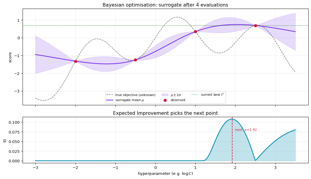
Bayesian optimisation keeps a surrogate: a cheap probabilistic model of score-as-a-function-of-hyperparameter, fitted to what has been observed. It then picks the next point by maximising an acquisition function over that surrogate.
The standard choice is Expected Improvement. With current best $f^*$, and a surrogate predicting mean $\mu(x)$ and standard deviation $\sigma(x)$:
$$\text{EI}(x) = (\mu(x) - f^*)\,\Phi(z) + \sigma(x)\,\phi(z), \qquad z = \frac{\mu(x) - f^*}{\sigma(x)}$$
$\Phi$ and $\phi$ are the normal CDF and PDF. The two terms are the whole idea:
- $(\mu - f^*)\Phi(z)$ — exploitation: go where the surrogate predicts a good score
- $\sigma\,\phi(z)$ — exploration: go where the surrogate is uncertain
A point is worth evaluating if it is probably good or poorly understood. Below, EI is computed by hand from a Gaussian process and checked term by term.
==============================================================================
  EXPECTED IMPROVEMENT, COMPUTED BY HAND
==============================================================================

Four observations so far
==============================================================================
    x = -2.00   score = -1.3206
    x = -0.50   score = -1.2475
    x =  1.00   score =  0.3411
    x =  2.50   score =  0.6880
  current best f* = 0.6880 at x = 2.50

Fit the surrogate and read off mu and sigma
==============================================================================

EI at three candidate points, term by term
==============================================================================
       x        mu    sigma        z    exploit    explore         EI
  --------------------------------------------------------------
   -1.29   -1.4759   0.2118  -10.215    -0.0000     0.0000     0.0000
    0.21   -0.5263   0.1992   -6.096    -0.0000     0.0000     0.0000
    3.20    0.4597   0.3853   -0.593    -0.0632     0.1290     0.0658
  --------------------------------------------------------------
  EI is maximised at x = 1.919  ->  evaluate there next

  At that point mu = 0.7367 (below f* = 0.6880) but
  sigma = 0.2030. It is chosen for what is NOT known about it.

Verify the two terms sum to the closed form
==============================================================================
  exploitation  (0.7367 - 0.6880) * Phi(0.2398) = +0.028951
  exploration   0.2030 * phi(0.2398)           = +0.078698
  sum = 0.107649   |  from array: 0.107649   |  MATCH: True
4. Successive halving: spend the budget unevenly
A different axis entirely. Instead of choosing which configurations to try, successive halving chooses how much to spend on each.
Start many configurations on a small budget — few trees, few epochs, a fraction of the data. Keep the best fraction, multiply their budget, repeat. Bad configurations are killed early and cheaply; only survivors get the expensive runs.
The arithmetic is what sells it: the total cost of all rungs is roughly the number of rungs times the budget of one rung, so you evaluate far more configurations than a full-budget search of the same cost.
==============================================================================
  SUCCESSIVE HALVING: THE BUDGET ARITHMETIC
==============================================================================
  start: 27 configurations at 100 resources each  (eta = 3)

   rung   configs   resource each   rung cost
  --------------------------------------------
      0        27             100       2,700
      1         9             300       2,700
      2         3             900       2,700
      3         1           2,700       2,700
  --------------------------------------------
  total                                10,800

  Running all 27 configurations at the FINAL budget (2,700) would cost 72,900
  Successive halving explores the same 27 configurations for 10,800
  -> 6.8x cheaper, and the winner still got the full budget.

  The assumption it rests on: a configuration that is bad at a small
  budget is bad at a large one. Usually true, not always -- some
  settings (low learning rates especially) look terrible early and win
  eventually. That failure mode is what Hyperband hedges against, by
  running several brackets with different starting budgets.
5. The warning that belongs on every search
Everything on this page increases the number of configurations you compare. That is the point — and it is also exactly the thing that inflates a reported score.
From [[cross-validation]]: the best of $n$ noisy estimates is biased upward, and the bias grows with $n$. A 5,000-configuration search does not just cost more compute; it produces a more optimistic winner. The score of the best configuration is not an estimate of its performance.
The fix is unchanged: the search belongs inside an inner loop, and the number you report comes from an outer loop that the search never touched. Below is what that costs and what it buys.
==============================================================================
  A TUNED SCORE IS NOT A PERFORMANCE ESTIMATE
==============================================================================

Random search, reported the usual way
==============================================================================
  40 configurations tried
  best params : C=1.313, gamma=0.03833
  best CV     : 0.8500   <- usually reported as 'our score'

The same search, scored from outside
==============================================================================
  outer folds : [0.8933 0.8133 0.8133 0.84  ]
  nested CV   : 0.8400   <- what to actually expect

  optimism    : +0.0100

  This problem HAS real signal, so both numbers are well above chance
  and the gap is smaller than the pure-noise case in the
  cross-validation walkthrough. The direction is the same, and it is
  the direction that matters: tuning and reporting on the same folds
  always flatters the result.

Cost
==============================================================================
  flat search  : 40 configs x 4 inner folds = 160 fits
  nested       : x 4 outer folds = 640 fits
  4x the compute, for a number you can defend.
6. What to take away
Grids multiply; random search does not. A grid's cost is the product over parameters, and it spends that cost re-testing the same few values on each axis. For the same budget, random search tests as many distinct values of the important parameter as it has evaluations.
The random-search guarantee is dimension-free. $1-(1-q)^n$ contains no term for the number of hyperparameters. Sixty draws, 95% chance of the top 5% — whether there are two knobs or twenty.
Bayesian optimisation buys adaptivity, and is worth it when fits are expensive. Expected Improvement is a sum of two readable terms: go where it is probably good, or where you do not know.
Successive halving buys a different thing — configurations per unit compute. It rests on bad-early implying bad-late, which is usually but not always true.
And all of it inflates the winner. More configurations means a more optimistic best score. Tune inside, report from outside.
Verified in this notebook
- Hand-computed grid scores match
GridSearchCV.best_score_exactly - $1-(1-q)^n$ matches simulation across five $(q, n)$ pairs to within 0.01
- On a five-knob objective where one knob dominates, random search beat a 6×6 grid on the great majority of 400 trials at equal budget
- Expected Improvement recomputed term by term from $\mu$, $\sigma$, and $f^*$ matches the array
- Successive halving's rung arithmetic against a full-budget search of the same configurations
- A 40-configuration random search reported flat vs nested
Where this connects
[[cross-validation]] supplies the inner and outer loops, and the reason the outer one is not optional. [[data-leakage]] is the other way a search result turns out to be fiction. [[optimisers-sgd-to-adam]] tunes inside a single fit, which is a different problem from the one on this page.
References
- Random Search for Hyper-Parameter Optimization
- Practical Bayesian Optimization of Machine Learning Algorithms
- Hyperband: A Novel Bandit-Based Approach to Hyperparameter Optimization