🎯 K-Means
Every model so far has been given labels. K-means is the first that is not: it is handed only the points and asked to find structure.
The objective is one line — put each point with the nearest centre, and place the centres so the total squared distance is as small as possible:
$$\min_{\{S_1,\dots,S_k\}} \;\; \sum_{j=1}^{k}\sum_{\mathbf{x}\in S_j}\lVert\mathbf{x}-\boldsymbol{\mu}_j\rVert^2$$
Finding the true optimum is NP-hard, so k-means uses Lloyd's algorithm: alternate two steps that each provably reduce the objective.
- Assign every point to its nearest centre.
- Update every centre to the mean of the points assigned to it.
Neither step can ever increase the objective, so the algorithm always converges — though not necessarily to the best answer. Every iteration is shown below with the distances and the means written out, and the result is checked against scikit-learn.
Display helpers ready: banner, step, check, expand, show_matrix, show_matmul, show_elementwise.
1. The Data
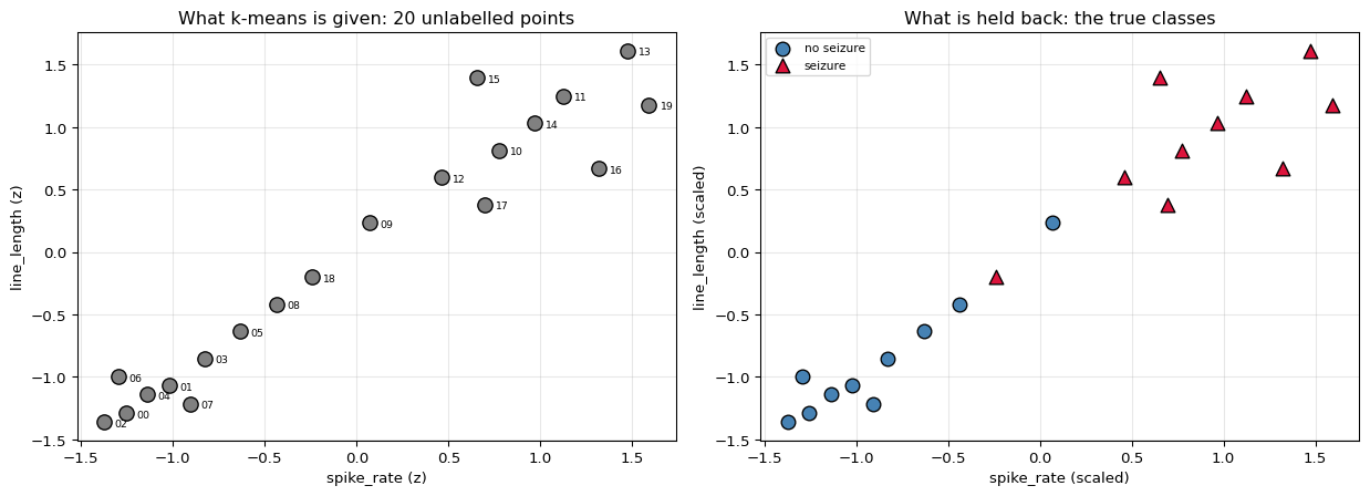
The same 20 EEG epochs used in the classification walkthroughs — but the labels are withheld. K-means never sees them.
They are kept aside for one purpose only: at the end we can ask whether the clusters the algorithm found happen to line up with the classes it was never told about.
20 epochs x 2 features, classes [10, 10]

    id   spike_rate   line_length   class         label
-------------------------------------------------------
  ep00          1.0          12.0       0    no seizure
  ep01          1.6          15.0       0    no seizure
  ep02          0.7          11.0       0    no seizure
  ep03          2.1          18.0       0    no seizure
  ep04          1.3          14.0       0    no seizure
  ep05          2.6          21.0       0    no seizure
  ep06          0.9          16.0       0    no seizure
  ep07          1.9          13.0       0    no seizure
  ep08          3.1          24.0       0    no seizure
  ep09          4.4          33.0       0    no seizure
  ep10          6.2          41.0       1       seizure
  ep11          7.1          47.0       1       seizure
  ep12          5.4          38.0       1       seizure
  ep13          8.0          52.0       1       seizure
  ep14          6.7          44.0       1       seizure
  ep15          5.9          49.0       1       seizure
  ep16          7.6          39.0       1       seizure
  ep17          6.0          35.0       1       seizure
  ep18          3.6          27.0       1       seizure
  ep19          8.3          46.0       1       seizure
-------------------------------------------------------

feature means : [ 4.22 29.75]
feature stds  : [ 2.564 13.794]

Note the scales: line_length spans ~41 while spike_rate spans ~8.
Any algorithm that measures DISTANCE will be dominated by the larger one
unless the features are scaled - that matters for KNN and SVM below.
Scaling matters here for the same reason it did for KNN: k-means minimises
SQUARED EUCLIDEAN distance, so an unscaled feature with a larger range
would dominate the objective and the clusters would only reflect it.
2. Initialisation
Lloyd's algorithm needs somewhere to start, and the starting point matters: the objective is non-convex, so different initialisations can converge to different answers.
Random init picks $k$ points at random. k-means++ spreads them out: the first centre is random, and each subsequent one is drawn with probability proportional to $D(\mathbf{x})^2$, the squared distance to the nearest centre already chosen. Far-away points are far more likely to be picked, which avoids starting with two centres on top of each other.
k-means++ initialisation:

   centre 1: chosen uniformly at random -> ep16
   centre 2: sampled with P proportional to D(x)^2
        ep02: D^2 = 11.3638, P = 0.1357  <- picked
        ep00: D^2 = 10.4586, P = 0.1249
        ep06: D^2 =  9.6099, P = 0.1147
        ep04: D^2 =  9.3232, P = 0.1113

starting centres:
   mu_0 = [1.3184 0.6706]   (at ep16)
   mu_1 = [-1.373  -1.3592]   (at ep02)

distance between them: 3.3710
a purely random pair would often be much closer, e.g. 0.2921
3. Lloyd's Algorithm, Iteration by Iteration
$$\text{assign: } \; c_i = \arg\min_j \lVert\mathbf{x}_i - \boldsymbol{\mu}_j\rVert^2 \qquad\qquad \text{update: } \; \boldsymbol{\mu}_j = \frac{1}{|S_j|}\sum_{i \in S_j}\mathbf{x}_i$$
The inertia (the objective being minimised) is printed after each step so the monotone decrease is visible:
$$\text{inertia} = \sum_i \lVert\mathbf{x}_i - \boldsymbol{\mu}_{c_i}\rVert^2$$
=========== ITERATION 1 ===========
centres now: mu_0 = [1.3184 0.6706],  mu_1 = [-1.373  -1.3592]

ASSIGN - squared distance to each centre

    id    d^2 to mu_0    d^2 to mu_1   nearest
------------------------------------------------
  ep00     10.45856        0.01895 *         1
  ep01      8.50428        0.20732 *         1
  ep02     11.36379        0.00000 *         1
  ep03      6.91999        0.55571 *         1
  ep04      9.32321        0.10207 *         1
  ep05      5.50636        1.07477 *         1
  ep06      9.60987        0.13747 *         1
  ep07      8.49577        0.24011 *         1
  ep08      4.26339        1.76450 *         1
  ep09      1.74717 *      4.62641           0
  ep10      0.31923 *      9.33213           0
  ep11      0.37437 *     13.04268           0
  ep12      0.74165 *      7.19197           0
  ep13      0.91247 *     16.94190           0
  ep14      0.25462 *     11.20020           0
  ep15      0.96522 *     11.70257           0
  ep16      0.00000 *     11.36379           0
  ep17      0.47358 *      7.30080           0
  ep18      3.19110        2.62489 *         1
  ep19      0.33206 *     15.22563           0
------------------------------------------------
cluster sizes: [10, 10]
inertia after assignment: 12.846152

UPDATE - each centre becomes the mean of its members

   cluster 0 (10 points): ['ep09', 'ep10', 'ep11', 'ep12', 'ep13', 'ep14', 'ep15', 'ep16', 'ep17', 'ep19']
      spike_rate: (+0.070 + +0.772 + +1.123 + +0.460 + +1.474 + +0.967 + ...) / 10 = +0.912740
      line_length: (+0.236 + +0.816 + +1.251 + +0.598 + +1.613 + +1.033 + ...) / 10 = +0.917034
      mu_0 : [1.3184 0.6706]  ->  [0.9127 0.917 ]
   cluster 1 (10 points): ['ep00', 'ep01', 'ep02', 'ep03', 'ep04', 'ep05', 'ep06', 'ep07', 'ep08', 'ep18']
      spike_rate: (-1.256 + -1.022 + -1.373 + -0.827 + -1.139 + -0.632 + ...) / 10 = -0.912740
      line_length: (-1.287 + -1.069 + -1.359 + -0.852 + -1.142 + -0.634 + ...) / 10 = -0.917034
      mu_1 : [-1.373  -1.3592]  ->  [-0.9127 -0.917 ]

   centre movement: [0.4747 0.6383]
   inertia after update: 6.519077  (was 12.846152)

=========== ITERATION 2 ===========
centres now: mu_0 = [0.9127 0.917 ],  mu_1 = [-0.9127 -0.917 ]

ASSIGN - squared distance to each centre

    id    d^2 to mu_0    d^2 to mu_1   nearest
------------------------------------------------
  ep00      9.56006        0.25451 *         1
  ep01      7.68845        0.03510 *         1
  ep02     10.40608        0.40740 *         1
  ep03      6.15518        0.01162 *         1
  ep04      8.44818        0.10168 *         1
  ep05      4.79258        0.15880 *         1
  ep06      8.53678        0.15248 *         1
  ep07      7.84635        0.08840 *         1
  ep08      3.60064        0.47666 *         1
  ep09      1.17421 *      2.29476           0
  ep10      0.03002 *      5.84125           0
  ep11      0.15557 *      8.84396           0
  ep12      0.30647 *      4.18069           0
  ep13      0.79981 *     12.09946           0
  ep14      0.01644 *      7.33745           0
  ep15      0.29519 *      7.80650           0
  ep16      0.22531 *      7.49845           0
  ep17      0.33549 *      4.26642           0
  ep18      2.57937        0.96517 *         1
  ep19      0.52875 *     10.66014           0
------------------------------------------------
cluster sizes: [10, 10]
inertia after assignment: 6.519077

UPDATE - each centre becomes the mean of its members

   cluster 0 (10 points): ['ep09', 'ep10', 'ep11', 'ep12', 'ep13', 'ep14', 'ep15', 'ep16', 'ep17', 'ep19']
      spike_rate: (+0.070 + +0.772 + +1.123 + +0.460 + +1.474 + +0.967 + ...) / 10 = +0.912740
      line_length: (+0.236 + +0.816 + +1.251 + +0.598 + +1.613 + +1.033 + ...) / 10 = +0.917034
      mu_0 : [0.9127 0.917 ]  ->  [0.9127 0.917 ]
   cluster 1 (10 points): ['ep00', 'ep01', 'ep02', 'ep03', 'ep04', 'ep05', 'ep06', 'ep07', 'ep08', 'ep18']
      spike_rate: (-1.256 + -1.022 + -1.373 + -0.827 + -1.139 + -0.632 + ...) / 10 = -0.912740
      line_length: (-1.287 + -1.069 + -1.359 + -0.852 + -1.142 + -0.634 + ...) / 10 = -0.917034
      mu_1 : [-0.9127 -0.917 ]  ->  [-0.9127 -0.917 ]

   centre movement: [0. 0.]
   inertia after update: 6.519077  (was 6.519077)

>>> centres stopped moving - CONVERGED after 2 iterations

final inertia: 6.519077
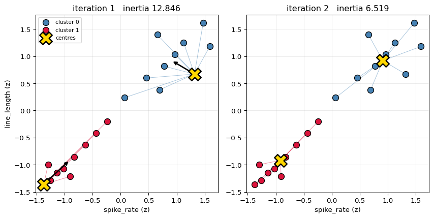
Black arrows show where each centre moves next. The thin lines are the
assignments whose squared lengths are being summed into the inertia.
Why it always converges
Each step is a minimisation of the same objective over a different variable:
- Assign holds the centres fixed and picks the best cluster for each point — by construction it cannot increase the total.
- Update holds the assignment fixed and picks the best centre for each cluster. The mean is exactly the minimiser of $\sum_{i\in S}\lVert\mathbf{x}_i-\boldsymbol{\mu}\rVert^2$, since $\frac{d}{d\mu}\sum(x_i-\mu)^2 = -2\sum(x_i-\mu) = 0 \Rightarrow \mu = \bar{x}$.
So the inertia is non-increasing and bounded below by zero. There are finitely many possible assignments, so it must stop.
What that argument does not promise is a good answer — only a stable one.
inertia after every half-step (never increases)

 step      kind       inertia        change
--------------------------------------------
    0    assign     12.846152
    1    update      6.519077     -6.327076
    2    assign      6.519077     +0.000000
    3    update      6.519077     +0.000000
--------------------------------------------

monotonically non-increasing throughout? True


verifying that the MEAN is the optimal centre for cluster 0:

   mean of the 10 members = [0.9127 0.917 ]
   sum of squared distances     = 3.86724640
   random nearby centres that do better: 0/5000
4. Local Minima
The objective is non-convex, so where you start decides where you land. Running Lloyd's
algorithm from many random initialisations and keeping the best is not a refinement — it
is a necessity, and it is what n_init does in scikit-learn.
200 random restarts, k = 2

  inertia reached    times     share
------------------------------------
         6.519077      200   100.0%
------------------------------------

distinct local minima found: 1
best: 6.519077   worst: 6.519077
on this small, well-separated data every restart found the same optimum;
with more clusters or messier data that stops being true - see k = 4 below.

k = 3: 6 distinct optima, best 3.6837, worst 4.7236  (best found 43% of the time)

k = 4: 46 distinct optima, best 2.2182, worst 4.3499  (best found 2% of the time)

k = 5: 109 distinct optima, best 1.6162, worst 3.5825  (best found 2% of the time)
5. Choosing $k$
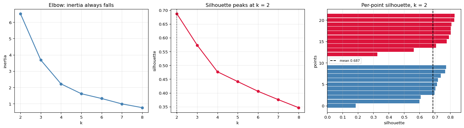
Inertia always falls as $k$ rises — at $k = n$ it reaches zero, with every point its own cluster. So it cannot be minimised to choose $k$.
Two standard alternatives:
The elbow. Plot inertia against $k$ and look for the bend where extra clusters stop buying much. It is a judgement call, not a criterion.
Silhouette. For each point compare $a$, its mean distance to its own cluster, with $b$, the mean distance to the nearest other cluster:
$$s = \frac{b - a}{\max(a, b)} \;\in\; [-1, 1]$$
Near $+1$ the point is comfortably inside its cluster; near $0$ it sits on a border; negative means it would be happier elsewhere.
k     inertia       drop   silhouette
----------------------------------------
   2      6.5191                  0.6868
   3      3.6837     2.8354       0.5733
   4      2.2182     1.4655       0.4767
   5      1.6162     0.6020       0.4410
   6      1.3230     0.2931       0.4060
   7      0.9921     0.3310       0.3757
   8      0.7635     0.2286       0.3467
----------------------------------------

best silhouette at k = 2 (0.6868)

lowest silhouettes at k = 2 (the border cases):
   ep09: s = +0.1858  (cluster 0, true class 0)
   ep18: s = +0.3259  (cluster 1, true class 1)
   ep08: s = +0.5625  (cluster 1, true class 0)
   ep17: s = +0.6003  (cluster 0, true class 1)
6. Did the Clusters Find the Classes?
K-means never saw a label, so cluster 0 has no reason to correspond to class 0 — the numbering is arbitrary. The comparison has to be made up to a permutation of labels, and the standard tool is the adjusted Rand index, which is 0 for random agreement and 1 for a perfect match.
cross-tabulation: true class vs discovered cluster

                 cluster 0   cluster 1
----------------------------------------
    no seizure           1           9
       seizure           9           1
----------------------------------------

agreement as-is        : 0.1000
agreement with labels flipped: 0.9000
best alignment         : 0.9000
adjusted Rand index    : 0.6200

disagreeing epochs: ['ep09', 'ep18']
those are the two planted overlaps - the same points logistic regression
and the SVM could not place either. Unsupervised or not, they sit in the
wrong neighbourhood.
What k-means cannot do
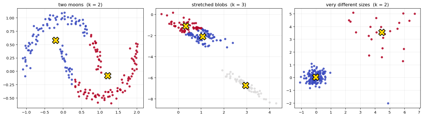
The objective assumes clusters are round, similarly sized, and separated by distance. When that is false, the algorithm still returns an answer — a confidently wrong one.
Left   : the moons are separated by SHAPE, not by distance to a centre.
Middle : stretched clusters get sliced across, because the objective is
         isotropic - it has no notion of a direction.
Right  : the large sparse cluster gets carved up to balance squared error.

All three failures come from the same source: minimising squared distance
to a single point per cluster can only ever produce convex, roughly
spherical regions. Density methods (DBSCAN) and Gaussian mixtures with
full covariance handle these; k-means structurally cannot.
7. Checking Against scikit-learn
our best over 200 restarts : inertia 6.51907675
sklearn (n_init=50)        : inertia 6.51907675
MATCH: True

centres (sorted so the arbitrary numbering lines up):
   ours [-0.9127 -0.917 ]   sklearn [-0.9127 -0.917 ]
   ours [0.9127 0.917 ]   sklearn [0.9127 0.917 ]

centres MATCH: True
assignments MATCH (up to relabelling): True

inertia recomputed from scratch: 6.51907675
sklearn's reported inertia_    : 6.51907675
MATCH: True
8. Summary
| Stage | Formula |
|---|---|
| Objective | $\sum_j\sum_{\mathbf{x}\in S_j}\lVert\mathbf{x}-\boldsymbol{\mu}_j\rVert^2$ |
| Assign | $c_i = \arg\min_j\lVert\mathbf{x}_i-\boldsymbol{\mu}_j\rVert^2$ |
| Update | $\boldsymbol{\mu}_j = \frac{1}{\lvert S_j\rvert}\sum_{i\in S_j}\mathbf{x}_i$ |
| Cost | $O(n\,k\,d)$ per iteration |
| Convergence | guaranteed — to a local optimum |
| Choosing $k$ | elbow, silhouette; never inertia alone |
The one idea: alternate between two steps that each minimise the same objective over one variable while holding the other fixed. Neither can make things worse, so the process must settle. That pattern — coordinate descent — recurs well beyond k-means; the EM algorithm for Gaussian mixtures is the same skeleton with soft assignments.
Its honest limits: you must choose $k$ in advance; the answer depends on initialisation; and clusters can only ever be round blobs of similar size, because a single mean per cluster cannot express anything else.
What is deliberately left out: k-medoids and k-medians, mini-batch k-means for large data, Gaussian mixture models (soft assignment plus covariance), DBSCAN and hierarchical clustering, and the formal proof of the $O(\log k)$ approximation guarantee that k-means++ provides.