📍 K-Nearest Neighbours
K-nearest neighbours has no training step and no parameters. It stores the data, and when asked to classify a point it looks at the $k$ closest stored examples and takes a vote.
That sounds too simple to be interesting, but three real ideas hide inside it:
- What "closest" means — the distance metric, and why unscaled features silently break it,
- What $k$ controls — a direct, visible bias/variance dial,
- Why it fails in high dimensions — the curse of dimensionality, which is easiest to demonstrate here.
Everything below computes the distance matrix explicitly, votes by hand, and checks the result against scikit-learn.
Display helpers ready: banner, step, check, expand, show_matrix, show_matmul, show_elementwise.
1. The Data
The same 20 EEG epochs used in the Logistic Regression walkthrough, so the decision boundaries can be compared side by side.
Look carefully at the two feature ranges printed below — that gap is about to matter more than anything else in this notebook.
20 epochs x 2 features, classes [10, 10]

    id   spike_rate   line_length   class         label
-------------------------------------------------------
  ep00          1.0          12.0       0    no seizure
  ep01          1.6          15.0       0    no seizure
  ep02          0.7          11.0       0    no seizure
  ep03          2.1          18.0       0    no seizure
  ep04          1.3          14.0       0    no seizure
  ep05          2.6          21.0       0    no seizure
  ep06          0.9          16.0       0    no seizure
  ep07          1.9          13.0       0    no seizure
  ep08          3.1          24.0       0    no seizure
  ep09          4.4          33.0       0    no seizure
  ep10          6.2          41.0       1       seizure
  ep11          7.1          47.0       1       seizure
  ep12          5.4          38.0       1       seizure
  ep13          8.0          52.0       1       seizure
  ep14          6.7          44.0       1       seizure
  ep15          5.9          49.0       1       seizure
  ep16          7.6          39.0       1       seizure
  ep17          6.0          35.0       1       seizure
  ep18          3.6          27.0       1       seizure
  ep19          8.3          46.0       1       seizure
-------------------------------------------------------

feature means : [ 4.22 29.75]
feature stds  : [ 2.564 13.794]

Note the scales: line_length spans ~41 while spike_rate spans ~8.
Any algorithm that measures DISTANCE will be dominated by the larger one
unless the features are scaled - that matters for KNN and SVM below.
2. Distance
The default is Euclidean distance:
$$d(\mathbf{a},\mathbf{b}) = \sqrt{\sum_j (a_j - b_j)^2}$$
Other choices change the shape of a "neighbourhood":
$$\text{Manhattan: } \sum_j |a_j - b_j| \qquad \text{Minkowski}_p: \Big(\sum_j |a_j-b_j|^p\Big)^{1/p} \qquad \text{Chebyshev: } \max_j |a_j - b_j|$$
Euclidean and Manhattan are Minkowski with $p = 2$ and $p = 1$.
a new epoch to classify: spike_rate = 4.0, line_length = 30.0

distance to ep00 = [ 1. 12.], worked out:
   d^2 = (4.0 - 1.0)^2 + (30.0 - 12.0)^2
       = (+3.0)^2 + (+18.0)^2
       = 9.00 + 324.00 = 333.00
   d   = sqrt(333.00) = 18.248288

   NOTICE: 324 of the 333 comes from line_length alone.
   spike_rate contributed 9.00 - essentially nothing.


all 20 distances from the query, sorted

 rank      id   spike_rate   line_length    distance   class
------------------------------------------------------------
    1    ep09          4.4          33.0      3.0265       0
    2    ep18          3.6          27.0      3.0265       1
    3    ep17          6.0          35.0      5.3852       1
    4    ep08          3.1          24.0      6.0671       0
    5    ep12          5.4          38.0      8.1216       1
    6    ep05          2.6          21.0      9.1082       0
    7    ep16          7.6          39.0      9.6933       1
    8    ep10          6.2          41.0     11.2178       1
    9    ep03          2.1          18.0     12.1495       0
   10    ep14          6.7          44.0     14.2580       1
   11    ep06          0.9          16.0     14.3391       0
   12    ep01          1.6          15.0     15.1908       0
   13    ep04          1.3          14.0     16.2262       0
   14    ep19          8.3          46.0     16.5677       1
   15    ep07          1.9          13.0     17.1292       0
   16    ep11          7.1          47.0     17.2803       1
   17    ep00          1.0          12.0     18.2483       0
   18    ep15          5.9          49.0     19.0948       1
   19    ep02          0.7          11.0     19.2844       0
   20    ep13          8.0          52.0     22.3607       1
------------------------------------------------------------
Scaling is not optional
line_length spans roughly 40 units; spike_rate spans roughly 7. Squared, that is a
factor of about 30. So Euclidean distance is almost entirely a measure of
line_length, and spike_rate is effectively ignored — not because it is
uninformative, but because it is measured in smaller numbers.
Standardising each feature to zero mean and unit variance puts them on equal terms:
$$z_j = \frac{x_j - \mu_j}{\sigma_j}$$
feature         mean         std
----------------------------------
spike_rate      4.2200      2.5637
line_length     29.7500     13.7945
----------------------------------

query raw        : [ 4. 30.]
query standardised: [-0.0858  0.0181]

how much each feature contributes to the squared distance, on average

     feature     raw share    scaled share
------------------------------------------
  spike_rate         3.4%          50.2%
 line_length        96.6%          49.8%
------------------------------------------


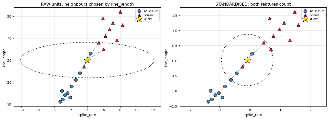
the 5 nearest neighbours change completely:

 rank            raw distance         scaled distance
------------------------------------------------------
    1     ep09 (d=3.027, c=0)     ep18 (d=0.268, c=1)
    2     ep18 (d=3.027, c=1)     ep09 (d=0.268, c=0)
    3     ep17 (d=5.385, c=1)     ep08 (d=0.559, c=0)
    4     ep08 (d=6.067, c=0)     ep12 (d=0.797, c=1)
    5     ep12 (d=8.122, c=1)     ep05 (d=0.851, c=0)
------------------------------------------------------

same 5 neighbours either way? False
The dotted circle is the k = 5 neighbourhood. On the left it is stretched by
the axis scales into something that only measures line_length; on the right
it is a genuine circle in a space where both features carry equal weight.
3. The Vote
$$\hat{y} = \arg\max_{c} \sum_{i \in N_k(\mathbf{x})} \mathbb{1}[\,y_i = c\,]$$
with $N_k$ the $k$ nearest stored points. Distance-weighted voting instead gives each neighbour a say proportional to $1/d$, so a very close neighbour outweighs a marginal one:
$$\hat{y} = \arg\max_{c} \sum_{i \in N_k} \frac{1}{d_i}\,\mathbb{1}[\,y_i = c\,]$$
query standardised = [-0.0858  0.0181]

k = 1:
   neighbours : ep18(c1,d=0.268)
   plain vote : class0 0, class1 1  ->  predict 1
   weighted   : class0 0.0000, class1 3.7361  ->  predict 1

k = 3:
   neighbours : ep18(c1,d=0.268), ep09(c0,d=0.268), ep08(c0,d=0.559)
   plain vote : class0 2, class1 1  ->  predict 0
   weighted   : class0 5.5252, class1 3.7361  ->  predict 0

k = 5:
   neighbours : ep18(c1,d=0.268), ep09(c0,d=0.268), ep08(c0,d=0.559), ep12(c1,d=0.797), ep05(c0,d=0.851)
   plain vote : class0 3, class1 2  ->  predict 0
   weighted   : class0 6.7005, class1 4.9915  ->  predict 0

k = 7:
   neighbours : ep18(c1,d=0.268), ep09(c0,d=0.268), ep08(c0,d=0.559), ep12(c1,d=0.797), ep05(c0,d=0.851), ep17(c1,d=0.860), ep03(c0,d=1.143)
   plain vote : class0 4, class1 3  ->  predict 0
   weighted   : class0 7.5756, class1 6.1540  ->  predict 0

k = 9:
   neighbours : ep18(c1,d=0.268), ep09(c0,d=0.268), ep08(c0,d=0.559), ep12(c1,d=0.797), ep05(c0,d=0.851), ep17(c1,d=0.860), ep03(c0,d=1.143), ep10(c1,d=1.171), ep01(c0,d=1.435)
   plain vote : class0 5, class1 4  ->  predict 0
   weighted   : class0 8.2725, class1 7.0076  ->  predict 0

the k = 5 weighted vote, written out:

   class 0: 1/0.2677 + 1/0.5590 + 1/0.8508 = 6.700538
   class 1: 1/0.2677 + 1/0.7966 = 4.991489

   -> predict class 0
4. What $k$ Controls
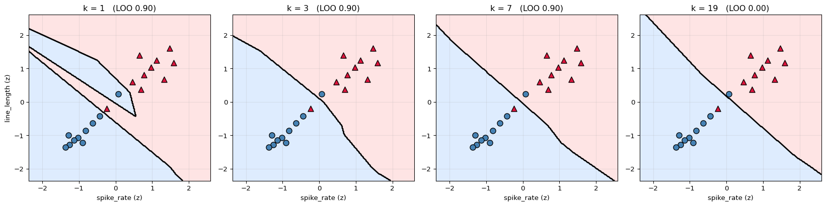
$k$ is a bias/variance dial, and unusually for machine learning you can see it:
- $k = 1$ — every training point gets its own island. Zero training error, maximum variance, and a boundary that contorts around individual noisy points.
- $k = n$ — every query gets the same answer, the majority class. Zero variance, maximum bias.
The interesting values are in between. Note that $k=1$ scoring 100% on training data is meaningless: the nearest neighbour of a training point is itself, at distance zero.
k   train acc   LOO-CV acc                                note
----------------------------------------------------------------
   1      1.0000       0.9000     each point is its own neighbour
   3      0.9000       0.9000
   5      0.9000       0.9000
   7      0.9000       0.9000
   9      0.9000       0.9000
  11      0.9000       0.9000
  15      0.9000       0.9000
  19      0.9000       0.0000          approaching majority-class
----------------------------------------------------------------

best k by leave-one-out CV: 1  (accuracy 0.9000)

Training accuracy is 1.0 at k=1 and tells us nothing. Leave-one-out
excludes the point itself, which is the only honest measure on 20 samples.
k = 1 carves separate pockets around the two awkward epochs - that is
variance. k = 19 has washed the boundary away entirely - that is bias.
5. The Curse of Dimensionality
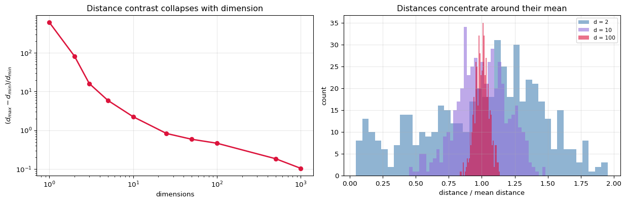
KNN rests on one assumption: near points have similar labels. In high dimensions that assumption quietly dies, because everything becomes equally far away.
For $n$ points spread in $d$ dimensions, the contrast between the nearest and farthest neighbour shrinks as $d$ grows:
$$\frac{d_{\max} - d_{\min}}{d_{\min}} \;\longrightarrow\; 0 \qquad \text{as } d \to \infty$$
Once that ratio approaches zero, "nearest" carries almost no information — the vote is close to random. This is the single most important limitation of the method, and it is easy to demonstrate.
500 uniform random points; distance from one query point

  dims      d_min      d_max       mean   (max-min)/min   std/mean
------------------------------------------------------------------
     1     0.0015     0.9159     0.4549        615.8064     0.6143
     2     0.0139     1.1548     0.6159         82.0189     0.4169
     3     0.0729     1.2504     0.6322         16.1509     0.3628
     5     0.2176     1.5075     0.8480          5.9276     0.2628
    10     0.6333     2.0570     1.3320          2.2480     0.1784
    25     1.5744     2.8810     2.2027          0.8299     0.1123
    50     2.2781     3.6173     2.9739          0.5879     0.0820
   100     3.2305     4.7314     4.2135          0.4646     0.0545
   500     8.2717     9.8038     9.1649          0.1852     0.0244
  1000    12.0941    13.3555    12.7334          0.1043     0.0178
------------------------------------------------------------------

In 1-D the farthest point is 616x further than the nearest.
In 1000-D it is only 0.10x further - every point sits at
almost exactly the same distance, so 'nearest' stops meaning anything.

Right panel: at d = 100 every distance is within a few percent of the mean.
The practical consequence: KNN needs either few dimensions, or a
dimensionality-reduction step first (see the PCA walkthrough).
6. Cost
There is no training cost at all — but every prediction rescans the dataset:
$$\text{train } O(1) \qquad\qquad \text{predict } O(n \cdot d) \text{ per query}$$
This is the opposite trade to every other model in this series, which pay up front and predict cheaply. Tree-based indexes (KD-tree, ball-tree) reduce the query cost to roughly $O(\log n)$ — but only in low dimensions. Above roughly 20 features they degrade to brute force, for exactly the reason shown in the previous section.
n      d    brute (ms)   kd_tree (ms)      winner
--------------------------------------------------------
    2000      2          13.9            2.2     kd_tree
    2000     20          15.2           19.2       brute
   20000      2          10.8            2.6     kd_tree
   20000     20           9.5          131.8       brute
   20000    100          15.1          679.9       brute
--------------------------------------------------------

kd_tree wins comfortably in 2-D and loses its advantage as d grows -
the same curse, showing up as a performance problem instead of an
accuracy problem.
7. Checking Against scikit-learn
k= 1  weights=uniform   MATCH: True
k= 1  weights=distance  MATCH: True
k= 3  weights=uniform   MATCH: True
k= 3  weights=distance  MATCH: True
k= 5  weights=uniform   MATCH: True
k= 5  weights=distance  MATCH: True
k= 7  weights=uniform   MATCH: True
k= 7  weights=distance  MATCH: True

the query point, k = 5:  ours 0, sklearn 0   MATCH: True

neighbour indices ours    : [18, 9, 8, 12, 5]
neighbour indices sklearn : [18, 9, 8, 12, 5]
MATCH: True

distances ours    : [0.267657, 0.267657, 0.558951, 0.796581, 0.850811]
distances sklearn : [0.267657, 0.267657, 0.558951, 0.796581, 0.850811]
MATCH: True
8. Summary
| Property | KNN |
|---|---|
| Training | none — the data is the model |
| Prediction | $O(n\cdot d)$ per query |
| Distance | $\sqrt{\sum_j (a_j-b_j)^2}$ (or Manhattan, Minkowski, …) |
| Vote | majority, or weighted by $1/d$ |
| $k$ small | low bias, high variance, jagged boundary |
| $k$ large | high bias, low variance, smooth boundary |
| Requires scaling | yes — unscaled features silently dominate |
| High dimensions | fails: distances concentrate |
The one idea: KNN makes no assumption about the shape of the boundary, which is its strength — it can represent anything. It assumes only that nearby points share labels, which is its weakness, because "nearby" depends entirely on the units you happened to measure in and collapses as dimensions grow.
What is deliberately left out: KD-tree and ball-tree construction, approximate nearest neighbours (HNSW, LSH) which is what makes vector search practical at scale, KNN regression (average instead of vote), learned metrics, and class-imbalance handling.