📈 Linear Regression
Linear regression is the one model whose optimum can be written down in closed form and verified by hand. Everything harder — logistic regression, SVMs, neural networks — replaces one piece of it and loses that closed form, so it is worth seeing exactly where the solution comes from.
The model is a weighted sum:
$$\hat{y}_i = w_0 + w_1 x_{i1} + \dots + w_p x_{ip} = \mathbf{x}_i^\top \mathbf{w}$$
and the loss is squared error:
$$\mathcal{L}(\mathbf{w}) = \sum_{i=1}^{n}(y_i - \mathbf{x}_i^\top\mathbf{w})^2 = \lVert \mathbf{y} - X\mathbf{w} \rVert^2$$
Below: the design matrix, $X^\top X$ and its inverse printed entry by entry, the normal equation solved by hand, the same answer reached again by gradient descent, then $R^2$, the residuals, and what ridge and lasso change. Every result is checked against scikit-learn.
Display helpers ready: banner, step, check, expand, show_matrix, show_matmul, show_elementwise.
1. The Data
12 EEG recordings. The target is y_reg — seizure burden in minutes per hour — and
the three features are the same ones used in the tree walkthroughs.
12 recordings x 3 features

    id      region   line_length    spike_rate           age   y_class    y_reg
-------------------------------------------------------------------------------
 rec00     frontal          12.0           0.5          24.0         0      0.2
 rec01    temporal          15.0           1.2          31.0         0      0.5
 rec02    temporal          42.0           6.8          58.0         1      6.4
 rec03   occipital          38.0           5.1          47.0         1      4.8
 rec04     frontal          11.0           0.3          19.0         0      0.1
 rec05    temporal          55.0           8.2          63.0         1      9.1
 rec06   occipital          40.0           1.9          35.0         1      3.5
 rec07    temporal          47.0           7.4          52.0         1      7.2
 rec08     frontal          14.0           0.8          28.0         0      0.3
 rec09   occipital          51.0           6.1          60.0         1      6.9
 rec10     frontal          45.0           2.4          41.0         0      1.6
 rec11    temporal          35.0           4.7          30.0         1      4.1
-------------------------------------------------------------------------------

class balance: 5 negative, 7 positive
y_reg mean = 3.7250, std = 3.0518
2. The Design Matrix
The intercept $w_0$ is handled by adding a column of ones. After that the intercept is just another weight and the whole model is a single matrix product:
$$\hat{\mathbf{y}} = X\mathbf{w}, \qquad X \in \mathbb{R}^{12 \times 4},\;\; \mathbf{w} \in \mathbb{R}^{4}$$
design matrix X: (12, 4)   (12 rows, 1 bias + 3 features)

    id      1 (bias)   line_length    spike_rate           age  |       y
-------------------------------------------------------------------------
 rec00          1.00         12.00          0.50         24.00  |    0.20
 rec01          1.00         15.00          1.20         31.00  |    0.50
 rec02          1.00         42.00          6.80         58.00  |    6.40
 rec03          1.00         38.00          5.10         47.00  |    4.80
 rec04          1.00         11.00          0.30         19.00  |    0.10
 rec05          1.00         55.00          8.20         63.00  |    9.10
 rec06          1.00         40.00          1.90         35.00  |    3.50
 rec07          1.00         47.00          7.40         52.00  |    7.20
 rec08          1.00         14.00          0.80         28.00  |    0.30
 rec09          1.00         51.00          6.10         60.00  |    6.90
 rec10          1.00         45.00          2.40         41.00  |    1.60
 rec11          1.00         35.00          4.70         30.00  |    4.10
-------------------------------------------------------------------------

the model has 4 unknowns and 12 equations - overdetermined,
so in general no w makes every residual zero. Least squares finds the w that
makes them as small as possible in the squared sense.
3. The Normal Equation
Write the loss in matrix form and differentiate:
$$\mathcal{L}(\mathbf{w}) = (\mathbf{y} - X\mathbf{w})^\top(\mathbf{y} - X\mathbf{w}) = \mathbf{y}^\top\mathbf{y} - 2\mathbf{w}^\top X^\top \mathbf{y} + \mathbf{w}^\top X^\top X \mathbf{w}$$
$$\frac{\partial \mathcal{L}}{\partial \mathbf{w}} = -2X^\top\mathbf{y} + 2X^\top X\mathbf{w} = 0$$
$$\boxed{\;\mathbf{w}^{*} = (X^\top X)^{-1} X^\top \mathbf{y}\;}$$
The loss is a convex quadratic, so this stationary point is the global minimum — there are no local minima to worry about and no learning rate to tune.
The geometry is worth holding onto: $X\mathbf{w}$ can only ever land in the column space of $X$. Least squares picks the point in that subspace closest to $\mathbf{y}$, which makes the residual orthogonal to every column of $X$. That orthogonality is checked numerically below.
STEP 1 : X^T X
==============================================================================
==============================================================================
  X^T (4, 12)   @   X (12, 4)   =   X^T X (4, 4)
==============================================================================
  shape rule: (4 x 12) @ (12 x 4) -> (4 x 4)   inner dim 12 cancels
  (4,12) @ (12,4) -> (4,4): a small square matrix, whatever n is
==============================================================================

X^T (4, 12) =
            0 |   +1.000    +1.000    +1.000    +1.000    +1.000    +1.000    +1.000    +1.000    +1.000    +1.000    +1.000    +1.000
            1 |  +12.000   +15.000   +42.000   +38.000   +11.000   +55.000   +40.000   +47.000   +14.000   +51.000   +45.000   +35.000
            2 |   +0.500    +1.200    +6.800    +5.100    +0.300    +8.200    +1.900    +7.400    +0.800    +6.100    +2.400    +4.700
            3 |  +24.000   +31.000   +58.000   +47.000   +19.000   +63.000   +35.000   +52.000   +28.000   +60.000   +41.000   +30.000

X (12, 4) =
            0 |   +1.000   +12.000    +0.500   +24.000
            1 |   +1.000   +15.000    +1.200   +31.000
            2 |   +1.000   +42.000    +6.800   +58.000
            3 |   +1.000   +38.000    +5.100   +47.000
            4 |   +1.000   +11.000    +0.300   +19.000
            5 |   +1.000   +55.000    +8.200   +63.000
            6 |   +1.000   +40.000    +1.900   +35.000
            7 |   +1.000   +47.000    +7.400   +52.000
            8 |   +1.000   +14.000    +0.800   +28.000
            9 |   +1.000   +51.000    +6.100   +60.000
           10 |   +1.000   +45.000    +2.400   +41.000
           11 |   +1.000   +35.000    +4.700   +30.000

X^T X (4, 4) =
            0 |  +12.000  +405.000   +45.400  +488.000
            1 | +405.000  +16579.000  +1976.300  +18840.000
            2 |  +45.400  +1976.300  +265.340  +2284.700
            3 | +488.000  +18840.000  +2284.700  +22334.000

  worked element  X^T X[0,0]  =  row 0 of X^T  .  column 0 of X
      row 0 of X^T = [1. 1. 1. 1. 1. 1. 1. 1. 1. 1. 1. 1.]
      col 0 of X = [1. 1. 1. 1. 1. 1. 1. 1. 1. 1. 1. 1.]
      (+1.0000)*(+1.0000) + (+1.0000)*(+1.0000) + (+1.0000)*(+1.0000) + (+1.0000)*(+1.0000) +
      (+1.0000)*(+1.0000) + (+1.0000)*(+1.0000) + (+1.0000)*(+1.0000) + (+1.0000)*(+1.0000) +
      (+1.0000)*(+1.0000) + (+1.0000)*(+1.0000) + (+1.0000)*(+1.0000) + (+1.0000)*(+1.0000)
      = +12.000000   |  from array: +12.000000   |  MATCH: True


STEP 2 : X^T y
==============================================================================
X^T y (1, 4) =
               1 (bias)line_lengthspike_rate       age
            0 |  +44.700  +2012.700  +268.720  +2300.200

   element 0 = sum of y            = 44.7000
   element 1 = sum of x1 * y        = 2012.7000
   check against the array          : True
STEP 3 : invert X^T X
==============================================================================
(X^T X)^-1 (4, 4) =
               1 (bias)line_lengthspike_rate       age
            0 |   +1.447993    -0.000838    +0.208314    -0.052242
            1 |   -0.000838    +0.001639    -0.002661    -0.001092
            2 |   +0.208314    -0.002661    +0.065530    -0.009011
            3 |   -0.052242    -0.001092    -0.009011    +0.003029

X^T X  @  (X^T X)^-1   (should be the identity) (4, 4) =
            0 |  +1.00000   +0.00000   +0.00000   -0.00000
            1 |  +0.00000   +1.00000   +0.00000   -0.00000
            2 |  -0.00000   +0.00000   +1.00000   -0.00000
            3 |  +0.00000   -0.00000   -0.00000   +1.00000

is it the identity? True
condition number of X^T X = 57,391.9

A large condition number means the inverse amplifies small changes in the
data into large changes in w - that is multicollinearity, and it is exactly
what ridge regression is built to control.
STEP 4 : w* = (X^T X)^-1 X^T y
==============================================================================
==============================================================================
  (X^T X)^-1 (4, 4)   @   X^T y (4, 1)   =   w* (4, 1)
==============================================================================
  shape rule: (4 x 4) @ (4 x 1) -> (4 x 1)   inner dim 4 cancels
==============================================================================

(X^T X)^-1 (4, 4) =
            0 |   +1.448    -0.001    +0.208    -0.052
            1 |   -0.001    +0.002    -0.003    -0.001
            2 |   +0.208    -0.003    +0.066    -0.009
            3 |   -0.052    -0.001    -0.009    +0.003

X^T y (4, 1) =
            0 |  +44.700
            1 | +2012.700
            2 | +268.720
            3 | +2300.200

w* (4, 1) =
            0 |   -1.150
            1 |   +0.034
            2 |   +0.839
            3 |   +0.013

  worked element  w*[0,0]  =  row 0 of (X^T X)^-1  .  column 0 of X^T y
      row 0 of (X^T X)^-1 = [ 1.448  -0.0008  0.2083 -0.0522]
      col 0 of X^T y = [  44.7  2012.7   268.72 2300.2 ]
      (+1.4480)*(+44.7000) + (-0.0008)*(+2012.7000) + (+0.2083)*(+268.7200) + (-0.0522)*(+2300.2000)
      = -1.149744   |  from array: -1.149744   |  MATCH: True


fitted coefficients

          term        weight
------------------------------
      1 (bias)     -1.149744
   line_length      0.034321
    spike_rate      0.839160
           age      0.013318
------------------------------

the fitted model:
   y_hat = -1.1497 +0.0343*line_length + +0.8392*spike_rate + +0.0133*age

Reading a coefficient: holding the other features fixed, one extra unit of
spike_rate is associated with +0.8392 more minutes of seizure burden.
'Associated with', not 'causes' - this is a correlational fit.
The residuals are orthogonal to the features
If the fit is truly optimal, no column of $X$ can explain any of what is left over:
$$X^\top(\mathbf{y} - X\mathbf{w}^{*}) = \mathbf{0}$$
Any non-zero entry here would mean some feature still carries unused signal — and the loss could be reduced further, contradicting optimality.
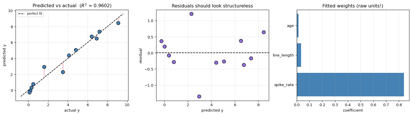
id         y      y_hat    residual
--------------------------------------
 rec00      0.20     0.0013      0.1987
 rec01      0.50     0.7849     -0.2849
 rec02      6.40     6.7705     -0.3705
 rec03      4.80     5.0601     -0.2601
 rec04      0.10    -0.2674      0.3674
 rec05      9.10     8.4580      0.6420
 rec06      3.50     2.2836      1.2164
 rec07      7.20     7.3657     -0.1657
 rec08      0.30     0.3750     -0.0750
 rec09      6.90     6.5186      0.3814
 rec10      1.60     2.9547     -1.3547
 rec11      4.10     4.3951     -0.2951
--------------------------------------
   SUM     44.70    44.7000    0.000000

X^T (y - Xw) = [0. 0. 0. 0.]
all zero (to numerical precision)? True

   the first entry is the sum of residuals - it is zero because of the
   bias column, which is why a model WITH an intercept always has
   residuals summing to zero: 8.76e-13
4. How Good Is the Fit?
$$R^2 = 1 - \frac{\sum_i (y_i - \hat y_i)^2}{\sum_i (y_i - \bar y)^2} = 1 - \frac{SS_{\text{res}}}{SS_{\text{tot}}}$$
$R^2$ compares the model against the simplest possible baseline: always predicting the mean. $R^2 = 0$ means the model is no better than that; $R^2 = 1$ means it fits perfectly.
A warning that matters here: $R^2$ never decreases when you add a feature, even a random one, because the extra column can only ever be used or ignored. Adjusted $R^2$ penalises that.
SS_res = sum of squared residuals   = 4.453102
SS_tot = sum of squared deviations  = 111.762500
         (from the mean y = 3.7250)

R^2      = 1 - 4.4531 / 111.7625 = 0.960156
adj. R^2 = 1 - (1 - 0.9602) * (12-1)/(12-3-1) = 0.945214

RMSE = sqrt(4.4531 / 12) = 0.609173 minutes/hour
MAE  = 0.467647

for scale: std(y) = 3.0518, so the model's typical error is
20.0% of the natural spread in the target.


adding a column of PURE NOISE, to show R^2 cannot fall:

   +1 random column(s): R^2 = 0.965113   adj R^2 =  0.945177
   +3 random column(s): R^2 = 0.982147   adj R^2 =  0.960723
   +6 random column(s): R^2 = 0.988970   adj R^2 =  0.939337

   R^2 climbs toward 1 with meaningless columns; adjusted R^2 turns back.
Middle panel: any visible pattern (a curve, a funnel) would mean the linear
form is wrong or the variance is not constant. With 12 points there is not
enough data to judge that seriously.

Right panel: these coefficients are in RAW units, so their sizes are not
comparable - age runs to 60 while spike_rate runs to 8. Comparing importance
requires standardising the features first.
5. How Learning Actually Happens
The closed form gave the answer in one step, which is convenient but hides the process. Every other model in this series — logistic regression, SVMs, neural networks — has to learn its weights by repeating one loop:
predict → measure the error → find which direction reduces it → take a small step → repeat
This section runs that loop with every number written out, so the mechanism is visible rather than asserted. To keep the arithmetic small enough to follow, it uses one feature plus a bias — two parameters, which also means the loss surface can be drawn.
The three pieces
1. The loss — how wrong we are right now (mean squared error):
$$\mathcal{L}(w_0, w_1) = \frac{1}{n}\sum_{i=1}^{n}\big(y_i - (w_0 + w_1 x_i)\big)^2$$
2. The derivatives — how the loss changes if each weight nudges up. Using the chain rule on $(y_i - w_0 - w_1x_i)^2$:
$$\frac{\partial\mathcal{L}}{\partial w_0} = \frac{2}{n}\sum_i \big(\hat{y}_i - y_i\big) \qquad\qquad \frac{\partial\mathcal{L}}{\partial w_1} = \frac{2}{n}\sum_i \big(\hat{y}_i - y_i\big)\,x_i$$
Read them directly: $\partial\mathcal{L}/\partial w_0$ is (twice) the average error — if predictions are too low overall, raise the intercept. $\partial\mathcal{L}/\partial w_1$ is (twice) the average error weighted by $x$ — if the errors are worse where $x$ is large, change the slope.
3. The update — step against the gradient, because the gradient points uphill:
$$w \leftarrow w - \eta\,\frac{\partial\mathcal{L}}{\partial w}$$
model      : y_hat = w0 + w1 * spike_rate
start at   : w0 = 0.0, w1 = 0.0   (predicting 0 for every recording)
learning rate eta = 0.02
loss at the start = 23.189167

for reference, the closed-form optimum for this 1-feature model is:
   w0* = -0.302061, w1* = +1.064421, loss* = 0.478401
Four epochs, every number
Each block below is one full pass: the current weights, what they predict for all 12 recordings, the error on each, the loss, both derivatives summed term by term, and the resulting update.
==============================================================================
  EPOCH 1      w0 = +0.000000      w1 = +0.000000
==============================================================================

STEP 1 - predict, and measure the error

    id        x        y    y_hat = w0 + w1*x   error (y_hat - y)    error^2
--------------------------------------------------------------------------
 rec00      0.5     0.20  +0.0000 + +0.0000*0.5 =  0.0000             -0.2000     0.0400
 rec01      1.2     0.50  +0.0000 + +0.0000*1.2 =  0.0000             -0.5000     0.2500
 rec02      6.8     6.40  +0.0000 + +0.0000*6.8 =  0.0000             -6.4000    40.9600
 rec03      5.1     4.80  +0.0000 + +0.0000*5.1 =  0.0000             -4.8000    23.0400
 rec04      0.3     0.10  +0.0000 + +0.0000*0.3 =  0.0000             -0.1000     0.0100
 rec05      8.2     9.10  +0.0000 + +0.0000*8.2 =  0.0000             -9.1000    82.8100
 rec06      1.9     3.50  +0.0000 + +0.0000*1.9 =  0.0000             -3.5000    12.2500
 rec07      7.4     7.20  +0.0000 + +0.0000*7.4 =  0.0000             -7.2000    51.8400
 rec08      0.8     0.30  +0.0000 + +0.0000*0.8 =  0.0000             -0.3000     0.0900
 rec09      6.1     6.90  +0.0000 + +0.0000*6.1 =  0.0000             -6.9000    47.6100
 rec10      2.4     1.60  +0.0000 + +0.0000*2.4 =  0.0000             -1.6000     2.5600
 rec11      4.7     4.10  +0.0000 + +0.0000*4.7 =  0.0000             -4.1000    16.8100
--------------------------------------------------------------------------
   loss = mean of the last column = 278.2700 / 12 = 23.189167

STEP 2 - the two derivatives

   dL/dw0 = (2/n) * sum(error)
          = (2/12) * (-0.200 + -0.500 + -6.400 + -4.800 + -0.100 + -9.100 + ...)
          = (2/12) * -44.700000
          = -7.450000

   dL/dw1 = (2/n) * sum(error * x)
          = (2/12) * (-0.10 + -0.60 + -43.52 + -24.48 + -0.03 + -74.62 + ...)
          = (2/12) * -268.720000
          = -44.786667

   both negative -> the loss falls if we INCREASE both weights

STEP 3 - step against the gradient

   w0 <- +0.000000 - 0.02 * (-7.450000) = +0.000000 +0.149000 = +0.149000
   w1 <- +0.000000 - 0.02 * (-44.786667) = +0.000000 +0.895733 = +0.895733

   loss: 23.189167  ->  0.735322   (DOWN by 22.453845)

==============================================================================
  EPOCH 2      w0 = +0.149000      w1 = +0.895733
==============================================================================

STEP 1 - predict, and measure the error

    id        x        y    y_hat = w0 + w1*x   error (y_hat - y)    error^2
--------------------------------------------------------------------------
 rec00      0.5     0.20  +0.1490 + +0.8957*0.5 =  0.5969              0.3969     0.1575
 rec01      1.2     0.50  +0.1490 + +0.8957*1.2 =  1.2239              0.7239     0.5240
 rec02      6.8     6.40  +0.1490 + +0.8957*6.8 =  6.2400             -0.1600     0.0256
 rec03      5.1     4.80  +0.1490 + +0.8957*5.1 =  4.7172             -0.0828     0.0068
 rec04      0.3     0.10  +0.1490 + +0.8957*0.3 =  0.4177              0.3177     0.1009
 rec05      8.2     9.10  +0.1490 + +0.8957*8.2 =  7.4940             -1.6060     2.5792
 rec06      1.9     3.50  +0.1490 + +0.8957*1.9 =  1.8509             -1.6491     2.7196
 rec07      7.4     7.20  +0.1490 + +0.8957*7.4 =  6.7774             -0.4226     0.1786
 rec08      0.8     0.30  +0.1490 + +0.8957*0.8 =  0.8656              0.5656     0.3199
 rec09      6.1     6.90  +0.1490 + +0.8957*6.1 =  5.6130             -1.2870     1.6564
 rec10      2.4     1.60  +0.1490 + +0.8957*2.4 =  2.2988              0.6988     0.4883
 rec11      4.7     4.10  +0.1490 + +0.8957*4.7 =  4.3589              0.2589     0.0671
--------------------------------------------------------------------------
   loss = mean of the last column = 8.8239 / 12 = 0.735322

STEP 2 - the two derivatives

   dL/dw0 = (2/n) * sum(error)
          = (2/12) * (+0.397 + +0.724 + -0.160 + -0.083 + +0.318 + -1.606 + ...)
          = (2/12) * -2.245707
          = -0.374284

   dL/dw1 = (2/n) * sum(error * x)
          = (2/12) * (+0.20 + +0.87 + -1.09 + -0.42 + +0.10 + -13.17 + ...)
          = (2/12) * -24.281517
          = -4.046920

   both negative -> the loss falls if we INCREASE both weights

STEP 3 - step against the gradient

   w0 <- +0.149000 - 0.02 * (-0.374284) = +0.149000 +0.007486 = +0.156486
   w1 <- +0.895733 - 0.02 * (-4.046920) = +0.895733 +0.080938 = +0.976672

   loss: 0.735322  ->  0.554464   (DOWN by 0.180858)

==============================================================================
  EPOCH 3      w0 = +0.156486      w1 = +0.976672
==============================================================================

STEP 1 - predict, and measure the error

    id        x        y    y_hat = w0 + w1*x   error (y_hat - y)    error^2
--------------------------------------------------------------------------
 rec00      0.5     0.20  +0.1565 + +0.9767*0.5 =  0.6448              0.4448     0.1979
 rec01      1.2     0.50  +0.1565 + +0.9767*1.2 =  1.3285              0.8285     0.6864
 rec02      6.8     6.40  +0.1565 + +0.9767*6.8 =  6.7979              0.3979     0.1583
 rec03      5.1     4.80  +0.1565 + +0.9767*5.1 =  5.1375              0.3375     0.1139
 rec04      0.3     0.10  +0.1565 + +0.9767*0.3 =  0.4495              0.3495     0.1221
 rec05      8.2     9.10  +0.1565 + +0.9767*8.2 =  8.1652             -0.9348     0.8739
 rec06      1.9     3.50  +0.1565 + +0.9767*1.9 =  2.0122             -1.4878     2.2137
 rec07      7.4     7.20  +0.1565 + +0.9767*7.4 =  7.3839              0.1839     0.0338
 rec08      0.8     0.30  +0.1565 + +0.9767*0.8 =  0.9378              0.6378     0.4068
 rec09      6.1     6.90  +0.1565 + +0.9767*6.1 =  6.1142             -0.7858     0.6175
 rec10      2.4     1.60  +0.1565 + +0.9767*2.4 =  2.5005              0.9005     0.8109
 rec11      4.7     4.10  +0.1565 + +0.9767*4.7 =  4.7468              0.6468     0.4184
--------------------------------------------------------------------------
   loss = mean of the last column = 6.6536 / 12 = 0.554464

STEP 2 - the two derivatives

   dL/dw0 = (2/n) * sum(error)
          = (2/12) * (+0.445 + +0.828 + +0.398 + +0.338 + +0.349 + -0.935 + ...)
          = (2/12) * +1.518725
          = +0.253121

   dL/dw1 = (2/n) * sum(error * x)
          = (2/12) * (+0.22 + +0.99 + +2.71 + +1.72 + +0.10 + -7.67 + ...)
          = (2/12) * -2.465474
          = -0.410912


STEP 3 - step against the gradient

   w0 <- +0.156486 - 0.02 * (+0.253121) = +0.156486 -0.005062 = +0.151423
   w1 <- +0.976672 - 0.02 * (-0.410912) = +0.976672 +0.008218 = +0.984890

   loss: 0.554464  ->  0.551009   (DOWN by 0.003454)

==============================================================================
  EPOCH 4      w0 = +0.151423      w1 = +0.984890
==============================================================================

STEP 1 - predict, and measure the error

    id        x        y    y_hat = w0 + w1*x   error (y_hat - y)    error^2
--------------------------------------------------------------------------
 rec00      0.5     0.20  +0.1514 + +0.9849*0.5 =  0.6439              0.4439     0.1970
 rec01      1.2     0.50  +0.1514 + +0.9849*1.2 =  1.3333              0.8333     0.6944
 rec02      6.8     6.40  +0.1514 + +0.9849*6.8 =  6.8487              0.4487     0.2013
 rec03      5.1     4.80  +0.1514 + +0.9849*5.1 =  5.1744              0.3744     0.1401
 rec04      0.3     0.10  +0.1514 + +0.9849*0.3 =  0.4469              0.3469     0.1203
 rec05      8.2     9.10  +0.1514 + +0.9849*8.2 =  8.2275             -0.8725     0.7612
 rec06      1.9     3.50  +0.1514 + +0.9849*1.9 =  2.0227             -1.4773     2.1824
 rec07      7.4     7.20  +0.1514 + +0.9849*7.4 =  7.4396              0.2396     0.0574
 rec08      0.8     0.30  +0.1514 + +0.9849*0.8 =  0.9393              0.6393     0.4087
 rec09      6.1     6.90  +0.1514 + +0.9849*6.1 =  6.1593             -0.7407     0.5487
 rec10      2.4     1.60  +0.1514 + +0.9849*2.4 =  2.5152              0.9152     0.8375
 rec11      4.7     4.10  +0.1514 + +0.9849*4.7 =  4.7804              0.6804     0.4630
--------------------------------------------------------------------------
   loss = mean of the last column = 6.6121 / 12 = 0.551009

STEP 2 - the two derivatives

   dL/dw0 = (2/n) * sum(error)
          = (2/12) * (+0.444 + +0.833 + +0.449 + +0.374 + +0.347 + -0.872 + ...)
          = (2/12) * +1.831084
          = +0.305181

   dL/dw1 = (2/n) * sum(error * x)
          = (2/12) * (+0.22 + +1.00 + +3.05 + +1.91 + +0.10 + -7.15 + ...)
          = (2/12) * -0.514678
          = -0.085780


STEP 3 - step against the gradient

   w0 <- +0.151423 - 0.02 * (+0.305181) = +0.151423 -0.006104 = +0.145320
   w1 <- +0.984890 - 0.02 * (-0.085780) = +0.984890 +0.001716 = +0.986606

   loss: 0.551009  ->  0.549023   (DOWN by 0.001987)
The same loop, continued to convergence
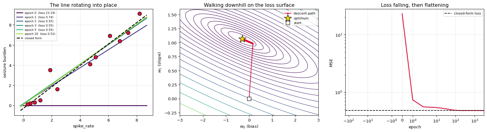
The gradient shrinks as the weights approach the optimum — at the minimum it is exactly zero, which is the same condition the normal equation solved directly in section 3.
epoch           w0           w1          loss       dL/dw0       dL/dw1   |gradient|
----------------------------------------------------------------------------------
      0     0.000000     0.000000     23.189167    -7.450000   -44.786667    4.540e+01
      1     0.149000     0.895733      0.735322    -0.374284    -4.046920    4.064e+00
      2     0.156486     0.976672      0.554464     0.253121    -0.410912    4.826e-01
      3     0.151423     0.984890      0.551009     0.305181    -0.085780    3.170e-01
      4     0.145320     0.986606      0.549023     0.305955    -0.056094    3.111e-01
      5     0.139201     0.987727      0.547101     0.302206    -0.052782    3.068e-01
     10     0.109793     0.992844      0.538249     0.282106    -0.049028    2.863e-01
     25     0.032815     1.006222      0.517968     0.229378    -0.039864    2.328e-01
     50    -0.064860     1.023197      0.498253     0.162475    -0.028237    1.649e-01
    100    -0.183051     1.043738      0.483398     0.081518    -0.014167    8.274e-02
    250    -0.287030     1.061809      0.478481     0.010296    -0.001789    1.045e-02
    500    -0.301583     1.064338      0.478401     0.000327    -0.000057    3.322e-04
   1000    -0.302060     1.064421      0.478401     0.000000    -0.000000    3.358e-07
   2000    -0.302061     1.064421      0.478401     0.000000    -0.000000    3.431e-13
   3000    -0.302061     1.064421      0.478401     0.000000    -0.000000    5.488e-15
----------------------------------------------------------------------------------
  exact    -0.302061     1.064421      0.478401            0            0            0

distance from the closed-form answer: 3.017e-15
MATCH with the normal equation: True

The gradient went from 45.40 to 5.49e-15. That is what 'converged'
means: there is no longer a direction that reduces the loss.
Middle panel: the path runs perpendicular to the contour lines - that IS
the gradient, which always points along the steepest direction. The steps
shorten near the optimum because the gradient itself is shrinking.
What the learning rate does
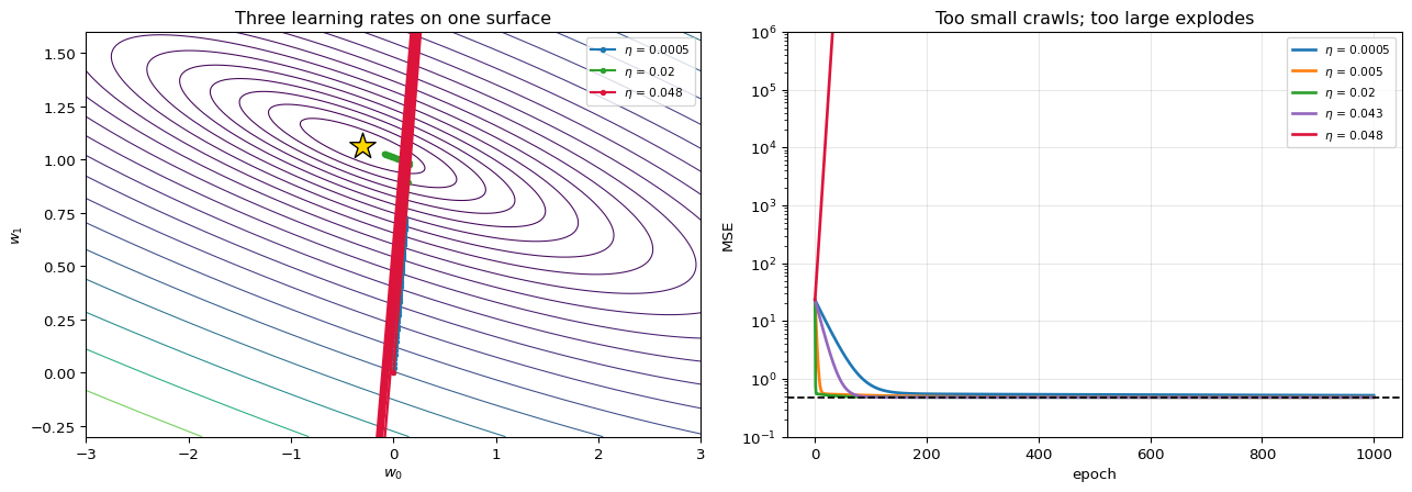
$\eta$ scales every step. The three failure modes are all visible on the same surface:
- too small — correct direction, but it crawls,
- about right — steady approach,
- too large — each step overshoots to a point further up the far wall, and the loss increases.
For squared error the boundary is knowable: descent is stable while $\eta < 2/\lambda_{\max}$, with $\lambda_{\max}$ the largest eigenvalue of the Hessian $\frac{2}{n}X^\top X$.
Hessian eigenvalues : [ 0.685  45.5384]
largest             : 45.538368
stable while eta    < 2 / 45.538368 = 0.04391901

         eta    vs limit      loss @10      loss @100     loss @1000       outcome
----------------------------------------------------------------------------------
      0.0005       0.01x       14.8346         0.7781         0.5182   still going
      0.0050       0.11x        0.6810         0.5181         0.4785     converged
      0.0200       0.46x        0.5382         0.4834         0.4784     converged
      0.0430       0.98x       10.1465         0.4830         0.4784     converged
      0.0480       1.09x      684.8322            inf            inf      DIVERGED
----------------------------------------------------------------------------------

The crimson run uses eta = 0.048, just above the limit of 0.04392,
and its loss grows without bound. Nothing is wrong with the gradient -
the direction is right every single step. The step length is the problem.
Batch, stochastic, and mini-batch
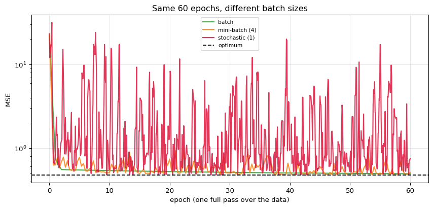
Every update above used all 12 recordings. Two cheaper variants trade accuracy per step for far more steps:
| Variant | Rows per update | Character |
|---|---|---|
| Batch | all $n$ | smooth, exact direction, expensive |
| Stochastic (SGD) | 1 | very noisy, very cheap |
| Mini-batch | 8–512 | the practical compromise |
The noise is not purely a cost. On a non-convex surface it can shake the parameters out of a poor basin — which is why essentially all deep learning uses mini-batches.
variant   rows/update    updates    final loss                     final w
----------------------------------------------------------------------------------
         batch            12         60      0.493467           [-0.0954  1.0285]
mini-batch (4)             4        180      0.513319           [-0.2844  1.0217]
    stochastic             1        720      0.752538           [-0.2737  0.9483]
----------------------------------------------------------------------------------
         exact             -          -      0.478401           [-0.3021  1.0644]
SGD makes 12 updates per epoch instead of 1, so it drops fastest at the
start - but it never settles, because each step follows a single recording
rather than the average. That permanent jitter is why real training
schedules decay the learning rate over time.
6. Scaling, and the Multi-Feature Case
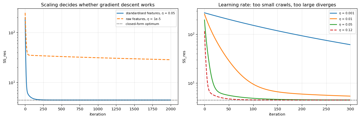
The step-by-step trace used one feature. With all three, one practical detail dominates:
feature scaling. age and spike_rate differ by an order of magnitude, which
stretches the loss surface into a long narrow valley and makes gradient descent zig-zag
across it instead of down it.
$$\nabla \mathcal{L} = -2X^\top(\mathbf{y} - X\mathbf{w}), \qquad \mathbf{w} \leftarrow \mathbf{w} - \eta \, \nabla\mathcal{L}$$
gradient descent on STANDARDISED features (eta = 0.05, 2000 steps)

          term   grad. descent    closed form        diff
----------------------------------------------------------
      1 (bias)        3.725000       3.725000    1.78e-15
   line_length        0.534488       0.534488    8.20e-09
    spike_rate        2.343354       2.343354    2.11e-08
           age        0.191786       0.191786    2.89e-08
----------------------------------------------------------

MATCH with the closed form: True
final SS_res: gradient descent 4.453102  vs  closed form 4.453102


same thing on RAW features - it needs eta = 1e-5 to stay stable,
and after the same 2000 steps it has still not converged:
   SS_res raw-feature GD  : 28.5471
   SS_res optimum         : 4.4531
   still 6.4x worse than optimal
The dashed curve on the right is past the stability limit and climbs away.
For least squares that limit is knowable: eta < 2 / largest eigenvalue of
(2/n) X^T X.
   largest eigenvalue = 5.5205  ->  stable for eta < 0.3623
7. Ridge and Lasso
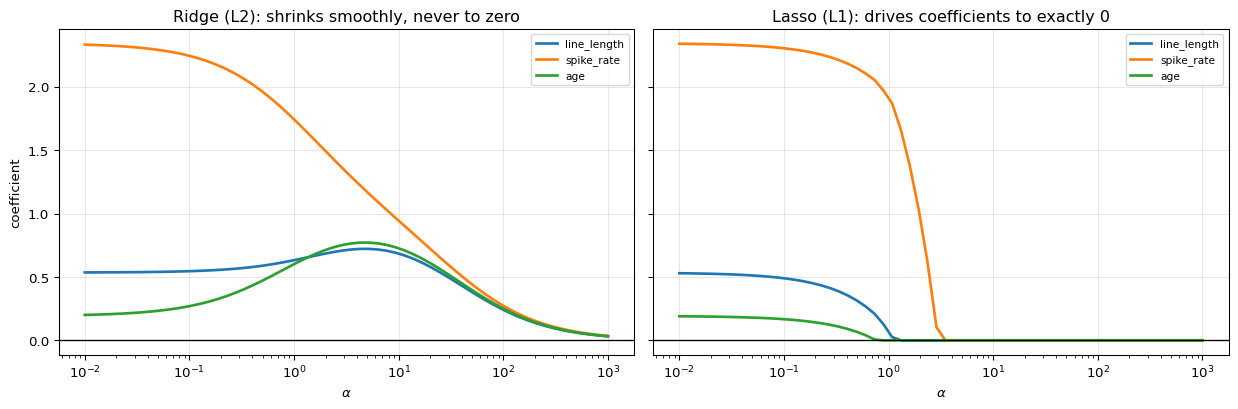
When features are correlated, $X^\top X$ is near-singular, its inverse blows up, and the fitted weights become large and unstable. Both remedies add a penalty on the size of $\mathbf{w}$:
$$\text{Ridge (L2):}\quad \lVert \mathbf{y} - X\mathbf{w}\rVert^2 + \alpha\lVert\mathbf{w}\rVert_2^2 \qquad\Longrightarrow\qquad \mathbf{w} = (X^\top X + \alpha I)^{-1}X^\top\mathbf{y}$$
$$\text{Lasso (L1):}\quad \lVert \mathbf{y} - X\mathbf{w}\rVert^2 + \alpha\lVert\mathbf{w}\rVert_1 \qquad\Longrightarrow\qquad \text{no closed form}$$
Ridge stays solvable in closed form — adding $\alpha I$ to the diagonal makes the matrix invertible again. Lasso does not, because $|w|$ is not differentiable at zero. That kink is precisely what drives coefficients to exactly zero, making lasso a feature selector while ridge only shrinks.
ridge, computed by hand from (X^T X + alpha I)^-1 X^T y
(the bias column is left unpenalised, as sklearn does)

   alpha   line_length    spike_rate           age      ||w||       R^2
--------------------------------------------------------------------------
     0.0       0.53449       2.34335       0.19179     2.4112   0.96016
     0.1       0.54538       2.24472       0.26955     2.3257   0.95998
     1.0       0.63211       1.74336       0.60086     1.9493   0.95355
    10.0       0.68444       0.94379       0.72615     1.3735   0.88587
   100.0       0.24061       0.27221       0.24989     0.4409   0.40543
--------------------------------------------------------------------------

our ridge (alpha=1) : [0.6321 1.7434 0.6009]
sklearn Ridge       : [0.6321 1.7434 0.6009]
MATCH: True
alpha    ridge: # exactly 0    lasso: # exactly 0
------------------------------------------------------
      0.1                     0                     0
      1.0                     0                     1
      5.0                     0                     3
     20.0                     0                     3
------------------------------------------------------

Ridge never reaches zero exactly; lasso does, and that is the whole
difference in one table.
8. Checking Against scikit-learn
term           ours        sklearn        diff
--------------------------------------------------------
     intercept    -1.14974437    -1.14974437    3.55e-15
   line_length     0.03432127     0.03432127    6.94e-18
    spike_rate     0.83915992     0.83915992    1.03e-14
           age     0.01331754     0.01331754    2.66e-15
--------------------------------------------------------

coefficients MATCH : True
predictions MATCH  : True
R^2 ours 0.96015567  sklearn 0.96015567  MATCH: True

vs np.linalg.lstsq (QR-based, more stable than inverting): True

In production never form (X^T X)^-1 explicitly - solve the system instead.
The inverse was written out here only because the point was to show it.
9. Summary
| Stage | Formula | Value here |
|---|---|---|
| Model | $\hat{\mathbf{y}} = X\mathbf{w}$ | 4 weights (bias + 3) |
| Loss | $\lVert\mathbf{y} - X\mathbf{w}\rVert^2$ | convex quadratic |
| Solution | $\mathbf{w}^{*} = (X^\top X)^{-1}X^\top\mathbf{y}$ | closed form, one step |
| Optimality | $X^\top(\mathbf{y} - X\mathbf{w}) = \mathbf{0}$ | verified to $10^{-9}$ |
| Fit | $R^2 = 1 - SS_{res}/SS_{tot}$ | see output above |
| Ridge | $(X^\top X + \alpha I)^{-1}X^\top\mathbf{y}$ | shrinks, never zeroes |
| Lasso | L1 penalty, iterative | zeroes coefficients |
The one idea: least squares is a projection. $X\mathbf{w}$ can only reach the column space of $X$, so the best it can do is the closest point in that subspace to $\mathbf{y}$ — which is why the residual comes out perpendicular to every feature.
What is deliberately left out: standard errors, $t$- and $p$-values, confidence intervals, the Gauss-Markov assumptions and what breaks when they fail, heteroscedasticity, weighted least squares, polynomial and spline bases, and elastic net.
What comes next: logistic regression keeps this exact linear form, $\mathbf{x}^\top\mathbf{w}$, and only changes what happens to it afterwards — a sigmoid instead of the identity, log-loss instead of squared error. That single change destroys the closed form and forces the iterative approach shown in section 5.