📉 Logistic Regression
Logistic regression keeps linear regression's core exactly — a weighted sum $z = \mathbf{x}^\top\mathbf{w}$ — and changes only what happens next.
Why change anything? Because a linear model outputs any real number, and a probability must lie in $[0,1]$. Fitting squared error to 0/1 labels gives predictions above 1 and below 0, and the loss is not even convex once squashed. Both problems are solved by the same substitution:
$$p = \sigma(z) = \frac{1}{1 + e^{-z}} \qquad\qquad \mathcal{L} = -\sum_i \big[\, y_i \log p_i + (1-y_i)\log(1-p_i) \,\big]$$
That pairing — sigmoid and log-loss — is not arbitrary. It produces a gradient of startling simplicity:
$$\nabla \mathcal{L} = X^\top(\mathbf{p} - \mathbf{y})$$
which is the same shape as the least-squares gradient, with predicted probabilities in place of predicted values. Everything below derives that, computes it by hand, runs both gradient descent and Newton's method, and checks the result against scikit-learn.
Display helpers ready: banner, step, check, expand, show_matrix, show_matmul, show_elementwise.
1. The Data
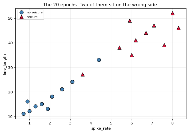
20 EEG epochs, two features, two classes. The same table is reused by the KNN, SVM and Naive Bayes walkthroughs so the decision boundaries can be compared directly.
Two epochs sit deliberately in the wrong region, so no straight line separates the classes perfectly. That matters: perfectly separable data makes logistic regression's weights diverge to infinity.
20 epochs x 2 features, classes [10, 10]

    id   spike_rate   line_length   class         label
-------------------------------------------------------
  ep00          1.0          12.0       0    no seizure
  ep01          1.6          15.0       0    no seizure
  ep02          0.7          11.0       0    no seizure
  ep03          2.1          18.0       0    no seizure
  ep04          1.3          14.0       0    no seizure
  ep05          2.6          21.0       0    no seizure
  ep06          0.9          16.0       0    no seizure
  ep07          1.9          13.0       0    no seizure
  ep08          3.1          24.0       0    no seizure
  ep09          4.4          33.0       0    no seizure
  ep10          6.2          41.0       1       seizure
  ep11          7.1          47.0       1       seizure
  ep12          5.4          38.0       1       seizure
  ep13          8.0          52.0       1       seizure
  ep14          6.7          44.0       1       seizure
  ep15          5.9          49.0       1       seizure
  ep16          7.6          39.0       1       seizure
  ep17          6.0          35.0       1       seizure
  ep18          3.6          27.0       1       seizure
  ep19          8.3          46.0       1       seizure
-------------------------------------------------------

feature means : [ 4.22 29.75]
feature stds  : [ 2.564 13.794]

Note the scales: line_length spans ~41 while spike_rate spans ~8.
Any algorithm that measures DISTANCE will be dominated by the larger one
unless the features are scaled - that matters for KNN and SVM below.
ep09: spike_rate=4.4, line_length=33.0, class 0 (no seizure)  <- the awkward one
   ep18: spike_rate=3.6, line_length=27.0, class 1 (seizure)  <- the awkward one
2. The Sigmoid and the Log-Odds
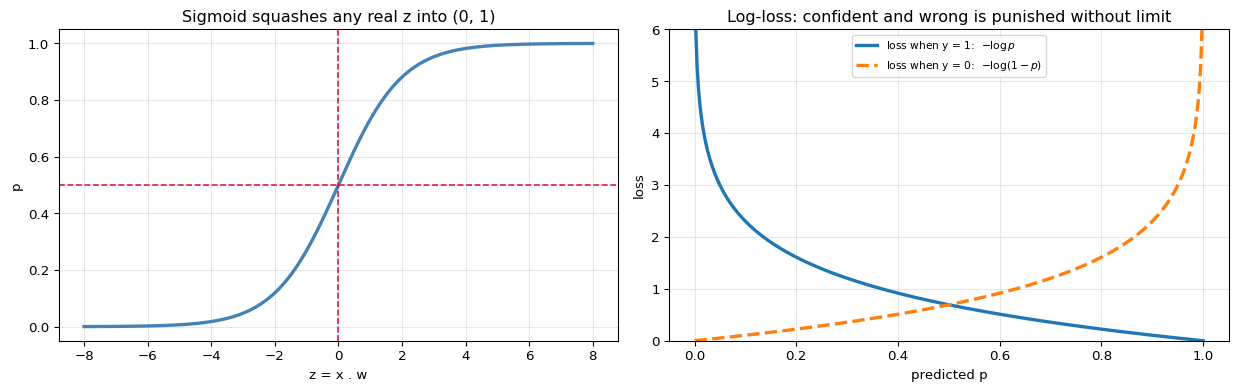
$$\sigma(z) = \frac{1}{1+e^{-z}}, \qquad \sigma'(z) = \sigma(z)\,(1-\sigma(z))$$
The inverse is the logit, and it is what the model is actually linear in:
$$z = \log\frac{p}{1-p} = \mathbf{x}^\top\mathbf{w}$$
So logistic regression asserts that the log-odds are a linear function of the features. A one-unit increase in $x_j$ multiplies the odds by $e^{w_j}$, whatever the starting point — which is why coefficients are usually reported as odds ratios.
z    sigma(z)     odds e^z   derivative
----------------------------------------------
   -6.0    0.002473       0.0025     0.002467
   -3.0    0.047426       0.0498     0.045177
   -2.0    0.119203       0.1353     0.104994
   -1.0    0.268941       0.3679     0.196612
   -0.5    0.377541       0.6065     0.235004
    0.0    0.500000       1.0000     0.250000
    0.5    0.622459       1.6487     0.235004
    1.0    0.731059       2.7183     0.196612
    2.0    0.880797       7.3891     0.104994
    3.0    0.952574      20.0855     0.045177
    6.0    0.997527     403.4288     0.002467
----------------------------------------------

sigma(0) = 0.500000   (odds 1:1, the decision boundary)
the derivative peaks at z = 0 with value 0.25 and vanishes at both ends -
that vanishing is why a very confident wrong prediction produces almost no
gradient, and why the Hessian below shrinks for confident points.

Right panel: as p -> 0 while y = 1, the loss goes to infinity. Squared error
would top out at 1. That unbounded penalty is what stops the model from
being confidently wrong.
3. Where the Gradient Comes From
This is the derivation worth doing once by hand. For a single sample, with $z = \mathbf{x}^\top\mathbf{w}$ and $p = \sigma(z)$:
$$\ell = -\big[y\log p + (1-y)\log(1-p)\big]$$
$$\frac{\partial \ell}{\partial p} = -\frac{y}{p} + \frac{1-y}{1-p} = \frac{p-y}{p(1-p)} \qquad\qquad \frac{\partial p}{\partial z} = p(1-p)$$
Multiply, and the awkward $p(1-p)$ cancels exactly:
$$\frac{\partial \ell}{\partial z} = \frac{p-y}{p(1-p)} \cdot p(1-p) = p - y$$
$$\boxed{\;\frac{\partial \ell}{\partial \mathbf{w}} = (p - y)\,\mathbf{x} \qquad\Longrightarrow\qquad \nabla\mathcal{L} = X^\top(\mathbf{p} - \mathbf{y})\;}$$
That cancellation is the whole reason log-loss is paired with the sigmoid. With squared error the $p(1-p)$ factor survives and multiplies the gradient by nearly zero whenever the model is confident — so a confidently wrong prediction would barely learn.
at w = 0, every prediction is p = 0.5 (maximum uncertainty)

    id         z         p     y      p - y
----------------------------------------
  ep00    0.0000    0.5000     0     0.5000
  ep01    0.0000    0.5000     0     0.5000
  ep02    0.0000    0.5000     0     0.5000
  ep03    0.0000    0.5000     0     0.5000
  ep04    0.0000    0.5000     0     0.5000
  ep05    0.0000    0.5000     0     0.5000
  ep06    0.0000    0.5000     0     0.5000
  ep07    0.0000    0.5000     0     0.5000
  ep08    0.0000    0.5000     0     0.5000
  ep09    0.0000    0.5000     0     0.5000
  ep10    0.0000    0.5000     1    -0.5000
  ep11    0.0000    0.5000     1    -0.5000
  ep12    0.0000    0.5000     1    -0.5000
  ep13    0.0000    0.5000     1    -0.5000
  ep14    0.0000    0.5000     1    -0.5000
  ep15    0.0000    0.5000     1    -0.5000
  ep16    0.0000    0.5000     1    -0.5000
  ep17    0.0000    0.5000     1    -0.5000
  ep18    0.0000    0.5000     1    -0.5000
  ep19    0.0000    0.5000     1    -0.5000
----------------------------------------

gradient = X^T (p - y):
       1 (bias):   0.000000
     spike_rate:  -8.815356
    line_length:  -8.735382

loss at w = 0 : 13.862944
   = -20 * log(0.5) = 13.862944   MATCH: True

That is the reference point every logistic model must beat: 20 samples
each contributing log(2) = 0.6931 nats of surprise.


comparing the two loss choices on a confidently WRONG prediction
(true y = 1, model says p = 0.01):

   log-loss      : -log(0.01) = 4.6052
   squared error : (1 - 0.01)^2 = 0.9801
   d(log-loss)/dz      = p - y = -0.9900
   d(squared err)/dz   = 2(p-y)p(1-p) = -0.019602

   the squared-error gradient is 51x smaller -
   it would barely correct this mistake.
4. Fitting by Gradient Descent
The loss is convex in $\mathbf{w}$, so there is a single global minimum — but unlike least squares there is no closed form, because setting $X^\top(\sigma(X\mathbf{w}) - \mathbf{y}) = 0$ gives an equation $\mathbf{w}$ cannot be factored out of. Iteration is the only option.
$$\mathbf{w} \leftarrow \mathbf{w} - \eta\, X^\top(\mathbf{p} - \mathbf{y})$$
first five gradient-descent steps, written out

 step        loss     1 (bias)   spike_rate  line_length
--------------------------------------------------------
    0   13.862944     0.000000     0.000000     0.000000
    1    7.971880     0.000000     0.440768     0.436769
    2    6.054044     0.000517     0.683642     0.675598
    3    5.147972     0.001729     0.847033     0.834818
    4    4.621426     0.003290     0.970285     0.953800
    5    4.277445     0.004997     1.069399     1.048574
--------------------------------------------------------

after 3000 steps:
       1 (bias):    0.379822
     spike_rate:    6.389715
    line_length:   -1.186748
   final loss: 2.669375   (started at 13.862944)
Newton's method (IRLS) — using the second derivative
Gradient descent only knows the slope. Newton's method also uses the curvature:
$$H = X^\top S X, \qquad S = \operatorname{diag}\big(p_i(1-p_i)\big)$$
$$\mathbf{w} \leftarrow \mathbf{w} - H^{-1}\nabla\mathcal{L}$$
Look at what $S$ contains: $p(1-p)$ is largest at $p = 0.5$ and near zero for confident predictions. Points the model is already sure about carry almost no weight — the fit is driven by the samples near the boundary. That is why this is called iteratively reweighted least squares, and it is the same idea that gives XGBoost its Hessian.
iter          loss     ||grad||    1 (bias)  spike_rate  line_length
------------------------------------------------------------------
    0   13.86294361    12.410375     0.00000     0.00000     0.00000
    1    4.88702047    12.410375    -0.00000     1.10555     0.68342
    2    3.36066270     3.113079     0.03329     2.11859     0.76908
    3    2.86124649     1.080105     0.10616     3.61054     0.27368
    4    2.69726818     0.353860     0.27274     5.67100    -0.92463
    5    2.64958943     0.112031     0.50127     7.65159    -2.20686
    6    2.64304583     0.036964     0.63540     8.65271    -2.83061
    7    2.64288765     0.005695     0.66018     8.83486    -2.94163
    8    2.64288754     0.000152     0.66084     8.83976    -2.94459
------------------------------------------------------------------

the IRLS weights S = p(1-p) at the solution:

    id          p    S = p(1-p)                     influence
--------------------------------------------------------------
  ep09    0.64285      0.229595  ######################
  ep18    0.29113      0.206371  ####################
  ep08    0.12201      0.107121  ##########
  ep15    0.91249      0.079853  #######
  ep12    0.95113      0.046483  ####
  ep05    0.04491      0.042891  ####
  ep07    0.02268      0.022170  ##
  ep03    0.01566      0.015415  #
  ep10    0.99386      0.006104
  ep01    0.00535      0.005326
  ep17    0.99659      0.003398
  ep04    0.00236      0.002358
  ep14    0.99791      0.002082
  ep00    0.00129      0.001287
  ep11    0.99900      0.000997
  ep02    0.00057      0.000567
  ep06    0.00039      0.000389
  ep13    0.99987      0.000130
  ep16    0.99997      0.000032
  ep19    0.99999      0.000013
--------------------------------------------------------------

The epochs at the top are the ones near the boundary - including the two
awkward ones. Confident points at the bottom contribute almost nothing.

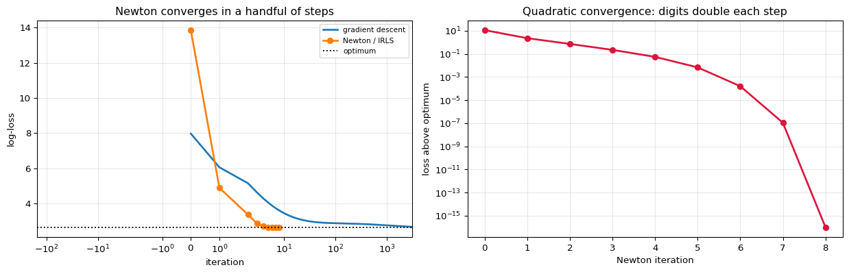
Newton reached loss 2.64288754 in 8 iterations;
gradient descent needed 3000 steps to reach 2.66937474.
iter      loss - optimum
--------------------------
    0           1.122e+01
    1           2.244e+00
    2           7.178e-01
    3           2.184e-01
    4           5.438e-02
    5           6.702e-03
    6           1.583e-04
    7           1.090e-07
    8           0.000e+00
--------------------------
Watching the boundary move
The weights are only numbers; what they mean is a line in feature space. Plotting the model at successive epochs turns the loss curve into something you can read directly.
epoch    w0 (bias)          w1          w2   loss/sample   accuracy
--------------------------------------------------------------------
      0     0.000000    0.000000    0.000000      0.693147     0.5000
      1     0.000000    0.440768    0.436769      0.398594     0.9000
      3     0.001729    0.847033    0.834818      0.257399     0.9000
     10     0.013500    1.392558    1.349501      0.176036     0.9000
     40     0.044748    2.063651    1.884941      0.147171     0.9000
    200     0.089106    2.769693    1.890634      0.142507     0.9000
   3000     0.379822    6.389715   -1.186748      0.133469     0.9000
--------------------------------------------------------------------

At epoch 0 every weight is zero, so the model predicts 0.5 everywhere -
the panel is uniformly pale and there is no boundary to draw. A usable
line appears almost immediately: accuracy is already 0.90 after ONE step.
Everything after that is the model chasing loss, not accuracy.
The boundary does NOT merely sharpen in place - it rotates. Note w2
changing sign between epoch 200 and 3000:
   cosine between the epoch-1 and epoch-3000 weight vectors = +0.5689
   i.e. about 55 degrees of rotation
With two epochs stranded on the wrong side, no line gets them right, so
the optimiser keeps trading confidence on one against the other - a lot
of weight movement buying very little loss.

   ||w|| at epoch 3    : 1.1893
   ||w|| at epoch 3000 : 6.5101
   accuracy at both    : 0.90 and 0.90

5. The Decision Boundary
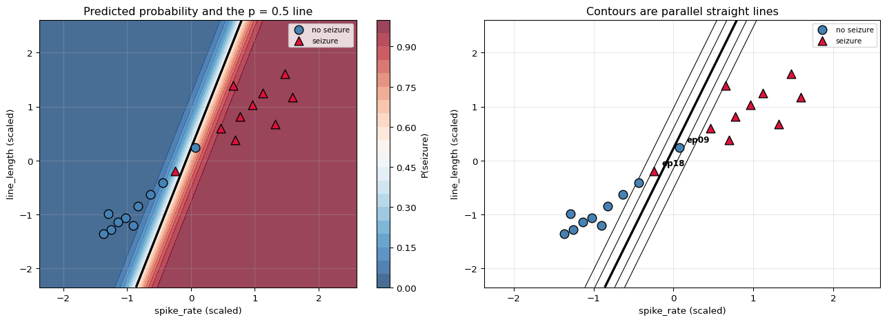
The boundary is where the model is undecided, $p = 0.5$, which means $z = 0$:
$$w_0 + w_1 x_1 + w_2 x_2 = 0 \qquad\Longrightarrow\qquad x_2 = -\frac{w_0 + w_1 x_1}{w_2}$$
A straight line — logistic regression is a linear classifier. What the sigmoid adds is not curvature but a graded confidence either side of that line.
boundary: +0.6608 +8.8398*spike_rate_z -2.9446*line_length_z = 0

    id          p   pred   true   correct
------------------------------------------
  ep00    0.00129      0      0       yes
  ep01    0.00535      0      0       yes
  ep02    0.00057      0      0       yes
  ep03    0.01566      0      0       yes
  ep04    0.00236      0      0       yes
  ep05    0.04491      0      0       yes
  ep06    0.00039      0      0       yes
  ep07    0.02268      0      0       yes
  ep08    0.12201      0      0       yes
  ep09    0.64285      1      0        NO
  ep10    0.99386      1      1       yes
  ep11    0.99900      1      1       yes
  ep12    0.95113      1      1       yes
  ep13    0.99987      1      1       yes
  ep14    0.99791      1      1       yes
  ep15    0.91249      1      1       yes
  ep16    0.99997      1      1       yes
  ep17    0.99659      1      1       yes
  ep18    0.29113      0      1        NO
  ep19    0.99999      1      1       yes
------------------------------------------

accuracy: 0.9000  (18/20)
misclassified: ['ep09', 'ep18']

Those are the two epochs planted on the wrong side. No straight line can
get them right - which is the honest limit of a linear classifier.
6. Reading the Coefficients as Odds Ratios
$$\text{odds} = \frac{p}{1-p} = e^{\mathbf{x}^\top\mathbf{w}} \qquad\Longrightarrow\qquad \text{one unit of } x_j \text{ multiplies the odds by } e^{w_j}$$
This is the property that keeps logistic regression in clinical use: the output is not just a prediction but a statement about how each variable changes the odds, and it holds at every point on the curve.
coefficients on STANDARDISED features, so one unit = one std dev

          term           w   odds ratio e^w                             reading
--------------------------------------------------------------------------------
      1 (bias)     0.66084          1.93642   odds at the mean of both features
    spike_rate     8.83976       6903.34132       +1 sd increases odds x6903.34
   line_length    -2.94459          0.05262          +1 sd decreases odds x0.05
--------------------------------------------------------------------------------

worked example, ep00:
   standardised features: [-1.256  -1.2867]
   z = (+1.0000)*(+0.6608) + (-1.2560)*(+8.8398) + (-1.2867)*(-2.9446)
     = -6.652896
   odds = e^-6.6529 = 0.001290
   p = odds/(1+odds) = 0.001289
   sigma(z)          = 0.001289   MATCH: True
7. What Regularisation Fixes
If the classes were perfectly separable, the likelihood would be maximised by pushing every $|w|$ toward infinity — the model can always make itself more certain, so no finite optimum exists. Adding a penalty bounds it:
$$\mathcal{L}_{\text{pen}} = -\sum_i\big[y_i\log p_i + (1-y_i)\log(1-p_i)\big] + \frac{1}{2C}\lVert\mathbf{w}\rVert^2$$
scikit-learn parameterises this as $C$, the inverse strength: small $C$ means heavy regularisation.
what happens on PERFECTLY separable data (no penalty)

  iterations         ||w||          loss
----------------------------------------
         100        3.2978     2.096e-01
         500        4.7129     4.429e-02
        2000        6.1124     1.221e-02
        8000        7.6226     3.331e-03
----------------------------------------

||w|| keeps growing and the loss keeps falling toward zero - there is no
finite optimum. The fit never converges; it only runs out of iterations.

with an L2 penalty the weights stay bounded:

         C       ||w||   train acc    spike_rate   line_length
--------------------------------------------------------------
      0.01      0.2158      1.0000       0.15286       0.15226
      0.10      0.6553      1.0000       0.46503       0.46169
      1.00      1.2278      1.0000       0.87470       0.86156
     10.00      1.9220      1.0000       1.37353       1.34448
   1000.00      3.7260      1.0000       2.95433       2.27040
--------------------------------------------------------------

That is what the penalty buys: a finite, stable answer even when the data
does not constrain the direction of w at all.
8. Checking Against scikit-learn
LogisticRegression(C=np.inf) optimises exactly the unpenalised loss derived above,
so the coefficients should agree with the hand-run Newton iteration.
term    ours (Newton)        sklearn         diff
------------------------------------------------------------
      1 (bias)       0.66083921     0.66083967     4.62e-07
    spike_rate       8.83976082     8.83976425     3.43e-06
   line_length      -2.94459034    -2.94459240     2.07e-06
------------------------------------------------------------

coefficients MATCH : True
probabilities MATCH: True
predictions MATCH  : True

log-loss ours    : 0.1321443769  (per sample)
log-loss sklearn : 0.1321443769
MATCH: True

gradient descent vs Newton (both ours):
   ||w_gd - w_newton|| = 3.028482e+00
   same solution? False
9. Summary
| Stage | Formula | Note |
|---|---|---|
| Linear part | $z = \mathbf{x}^\top\mathbf{w}$ | identical to linear regression |
| Link | $p = \sigma(z) = 1/(1+e^{-z})$ | maps $\mathbb{R} \to (0,1)$ |
| Loss | $-\sum y\log p + (1-y)\log(1-p)$ | convex, unbounded when wrong |
| Gradient | $X^\top(\mathbf{p}-\mathbf{y})$ | the $p(1-p)$ cancels |
| Hessian | $X^\top S X$, $S = \mathrm{diag}(p(1-p))$ | down-weights confident points |
| Boundary | $\mathbf{x}^\top\mathbf{w} = 0$ | a straight line |
| Coefficient | $e^{w_j}$ | odds ratio |
The one idea: the sigmoid and log-loss are chosen together. Either alone is awkward; paired, the derivative collapses to $p - y$ and the problem stays convex.
Its honest limit: the boundary is linear. The two planted epochs are misclassified and no amount of fitting will fix that — it needs a non-linear model, which is what the SVM-with-kernel and neural-network walkthroughs provide.
What is deliberately left out: multinomial/softmax regression, L1-penalised logistic regression, class weights for imbalanced data, calibration, ROC/AUC analysis, and the statistical machinery (Wald tests, deviance, confidence intervals on odds ratios).
References
- Pattern Recognition and Machine Learning, ch. 4