🎲 Naive Bayes
Every classifier so far has drawn a boundary directly. Naive Bayes takes the opposite route: it models how each class generates data, then applies Bayes' rule to invert that into a prediction.
$$P(y \mid \mathbf{x}) = \frac{P(\mathbf{x} \mid y)\,P(y)}{P(\mathbf{x})} \;\;\propto\;\; P(\mathbf{x}\mid y)\,P(y)$$
The obstacle is $P(\mathbf{x}\mid y)$: a joint distribution over all $p$ features needs exponentially much data to estimate. The "naive" assumption cuts it down to size by declaring the features conditionally independent given the class:
$$P(\mathbf{x}\mid y) = \prod_{j=1}^{p} P(x_j \mid y)$$
That turns one $p$-dimensional density into $p$ one-dimensional ones. The assumption is usually false — here the two EEG features correlate above 0.9 — and the classifier often works anyway. Section 6 shows precisely why.
Display helpers ready: banner, step, check, expand, show_matrix, show_matmul, show_elementwise.
1. The Data
The same 20 EEG epochs as the Logistic Regression, KNN and SVM walkthroughs, so all four decision boundaries can be compared on identical points.
20 epochs x 2 features, classes [10, 10]

    id   spike_rate   line_length   class         label
-------------------------------------------------------
  ep00          1.0          12.0       0    no seizure
  ep01          1.6          15.0       0    no seizure
  ep02          0.7          11.0       0    no seizure
  ep03          2.1          18.0       0    no seizure
  ep04          1.3          14.0       0    no seizure
  ep05          2.6          21.0       0    no seizure
  ep06          0.9          16.0       0    no seizure
  ep07          1.9          13.0       0    no seizure
  ep08          3.1          24.0       0    no seizure
  ep09          4.4          33.0       0    no seizure
  ep10          6.2          41.0       1       seizure
  ep11          7.1          47.0       1       seizure
  ep12          5.4          38.0       1       seizure
  ep13          8.0          52.0       1       seizure
  ep14          6.7          44.0       1       seizure
  ep15          5.9          49.0       1       seizure
  ep16          7.6          39.0       1       seizure
  ep17          6.0          35.0       1       seizure
  ep18          3.6          27.0       1       seizure
  ep19          8.3          46.0       1       seizure
-------------------------------------------------------

feature means : [ 4.22 29.75]
feature stds  : [ 2.564 13.794]

Note the scales: line_length spans ~41 while spike_rate spans ~8.
Any algorithm that measures DISTANCE will be dominated by the larger one
unless the features are scaled - that matters for KNN and SVM below.
correlation between the two features: +0.9621
   within class 0: +0.9489
   within class 1: +0.7524

Naive Bayes will assume these are ZERO. They are not. Keep that in mind
for section 6, where the consequence is measured.
2. Priors
$$P(y = c) = \frac{n_c}{n}$$
The prior is what the model believes before seeing any features — the base rate. On badly imbalanced data it dominates: if a condition affects 1 in 1000, the evidence must be strong to overcome a prior of 0.001.
class    count      prior    log prior
----------------------------------------------
    no seizure       10   0.500000    -0.693147
       seizure       10   0.500000    -0.693147
----------------------------------------------
         total       20   1.000000

Balanced here, so the prior will not decide anything. The formulas below
keep it explicit anyway, because on imbalanced data it does the deciding.
3. Per-Feature Likelihoods
For continuous features, Gaussian Naive Bayes fits one normal distribution per (feature, class) pair:
$$P(x_j \mid y=c) = \frac{1}{\sqrt{2\pi\sigma_{jc}^2}} \exp\!\left(-\frac{(x_j - \mu_{jc})^2}{2\sigma_{jc}^2}\right)$$
With $p$ features and $k$ classes that is $2pk$ numbers — here $2 \times 2 \times 2 = 8$. Modelling the full joint would instead require a $2\times2$ covariance matrix per class, and in higher dimensions the gap becomes the whole argument for the method.
Note the variance is the maximum-likelihood one (divide by $n_c$, not $n_c - 1$), which is what scikit-learn uses.
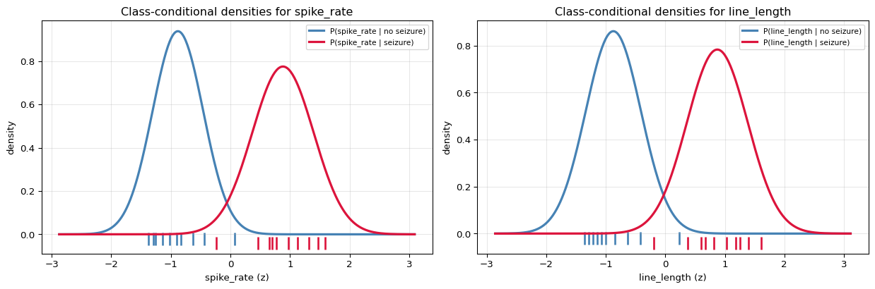
fitted parameters (standardised features)

         class       feature           mu      sigma^2       sigma
----------------------------------------------------------------
    no seizure    spike_rate    -0.881536     0.180811    0.425219
    no seizure   line_length    -0.873538     0.214465    0.463104
       seizure    spike_rate     0.881536     0.264979    0.514761
       seizure   line_length     0.873538     0.259397    0.509310
----------------------------------------------------------------

by hand, mu for class 0 / spike_rate:
   (-1.256 + -1.022 + -1.373 + -0.827 + -1.139 + ...) / 10
   = -8.815356 / 10 = -0.881536
   from the table: -0.881536   MATCH: True

   sigma^2 = sum (x - mu)^2 / n_c
           = (0.140 + 0.020 + 0.242 + 0.003 + 0.066 + ...) / 10
           = 1.808112 / 10 = 0.180811
   from the table: 0.180811   MATCH: True


total parameters: 2 classes x 2 features x (mu, sigma^2) = 8, plus 2 priors
a full joint Gaussian would need 2 classes x (2 means + 3 covariance terms) = 10
at p = 100 features: naive needs 400 numbers, full joint needs 10,300
Each panel is one row of the parameter table above. Naive Bayes multiplies
these two panels together and never asks whether that is legitimate.
4. Classifying One Point, By Hand
Work in log space. Multiplying many small probabilities underflows to zero in floating point; adding logs does not, and the arg max is unchanged:
$$\log P(y=c\mid\mathbf{x}) = \log P(y=c) + \sum_j \log P(x_j\mid y=c) - \log P(\mathbf{x})$$
The last term is the same for every class, so it can be ignored for the decision — but it is needed to turn the scores back into probabilities.
classifying ep09: spike_rate_z = +0.0702, line_length_z = +0.2356   (true class 0)

--- class 0 (no seizure) ---
   log P(y=0)                 = log(0.5000) = -0.693147
   P(spike_rate=+0.070 | y=0)
      = exp(-(+0.0702 - -0.8815)^2 / (2*0.1808)) / sqrt(2*pi*0.1808)
      = 0.07663754      log = -2.568668
   P(line_length=+0.236 | y=0)
      = exp(-(+0.2356 - -0.8735)^2 / (2*0.2145)) / sqrt(2*pi*0.2145)
      = 0.04893898      log = -3.017181
   log posterior (unnormalised) = -6.278997

--- class 1 (seizure) ---
   log P(y=1)                 = log(0.5000) = -0.693147
   P(spike_rate=+0.070 | y=1)
      = exp(-(+0.0702 - +0.8815)^2 / (2*0.2650)) / sqrt(2*pi*0.2650)
      = 0.22380903      log = -1.496962
   P(line_length=+0.236 | y=1)
      = exp(-(+0.2356 - +0.8735)^2 / (2*0.2594)) / sqrt(2*pi*0.2594)
      = 0.35747798      log = -1.028682
   log posterior (unnormalised) = -3.218791

normalising with the log-sum-exp trick (max = -3.218791):
   class 0: exp(-6.278997 - (-3.218791)) = 0.04687805
   class 1: exp(-3.218791 - (-3.218791)) = 1.00000000
   sum = 1.04687805
   P(y=0 | x) = 0.04477891
   P(y=1 | x) = 0.95522109

prediction: class 1   true: 0   WRONG
id    log P(.|0)    log P(.|1)    P(y=1|x)   pred   true    ok
----------------------------------------------------------------
  ep00      -1.69188     -18.80931    0.000000      0      0   yes
  ep01      -1.04991     -15.30473    0.000001      0      0   yes
  ep02      -2.12401     -20.39297    0.000000      0      0   yes
  ep03      -0.91542     -12.43781    0.000010      0      0   yes
  ep04      -1.25707     -16.72426    0.000000      0      0   yes
  ep05      -1.21182      -9.89677    0.000169      0      0   yes
  ep06      -1.41421     -16.87400    0.000000      0      0   yes
  ep07      -1.17823     -15.61638    0.000001      0      0   yes
  ep08      -1.93913      -7.68161    0.003197      0      0   yes
  ep09      -6.27900      -3.21879    0.955221      1      0    NO
  ep10     -15.12129      -1.22126    0.999999      1      1   yes
  ep11     -22.53982      -1.57654    1.000000      1      1   yes
  ep12     -10.93375      -1.67341    0.999905      1      1   yes
  ep13     -30.66935      -2.90946    1.000000      1      1   yes
  ep14     -18.83346      -1.25520    1.000000      1      1   yes
  ep15     -19.44043      -1.81397    1.000000      1      1   yes
  ep16     -19.84801      -1.63182    1.000000      1      1   yes
  ep17     -11.43999      -1.72682    0.999940      1      1   yes
  ep18      -3.09734      -5.79233    0.063270      0      1    NO
  ep19     -27.63014      -2.32193    1.000000      1      1   yes
----------------------------------------------------------------

accuracy: 0.9000  (18/20)
misclassified: ['ep09', 'ep18']
5. The Decision Boundary
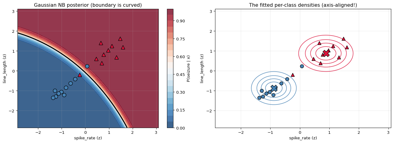
With equal variances across classes the log-posterior difference is linear in $\mathbf{x}$ and the boundary is a straight line. When the variances differ, the quadratic terms survive and the boundary becomes a conic — a parabola, ellipse or hyperbola.
So Gaussian Naive Bayes is a quadratic classifier in general, and reduces to a linear one in a special case.
variances per class:
   class 0: [0.1808 0.2145]   equal across features
   class 1: [0.265  0.2594]   equal across features

class variances identical across classes? False  -> boundary is quadratic

Right panel: the contours are ellipses aligned with the AXES. They can
never tilt, because a diagonal covariance has no off-diagonal term. The
real data is tilted, and that mismatch is the naive assumption made visible.
6. What the Naive Assumption Costs
The features here correlate above 0.9, so the independence assumption is plainly wrong. What does that cost?
The key insight: the assumption corrupts the probabilities much more than it corrupts the decision. Getting the arg max right only requires the ranking of the classes to survive, and that is far more robust than the magnitudes.
Below, Gaussian NB (diagonal covariance) is compared with QDA, which fits the full covariance and therefore makes no independence assumption.
model   train acc     LOO-CV   mean max prob
--------------------------------------------------------------------
   Gaussian NB (independent)      0.9000     0.9000        0.994421
       QDA (full covariance)      0.9000     0.9000        0.972994
--------------------------------------------------------------------

agreement between the two on which class wins: 100.0%
mean |difference| in P(y=1|x)                : 0.0214
max  |difference| in P(y=1|x)                : 0.2443

    id    NB P(y=1)    QDA P(y=1)       diff   same call?
--------------------------------------------------------
  ep09     0.955221      0.710928     0.2443         True
  ep18     0.063270      0.151356     0.0881         True
  ep08     0.003197      0.041183     0.0380         True
  ep12     0.999905      0.974879     0.0250         True
  ep17     0.999940      0.986978     0.0130         True
  ep05     0.000169      0.010498     0.0103         True
  ep10     0.999999      0.996773     0.0032         True
  ep03     0.000010      0.002681     0.0027         True
--------------------------------------------------------

predictions more extreme than 1% / 99%:
   Gaussian NB : 90.0%
   QDA         : 70.0%

NB is over-confident: multiplying correlated features counts the SAME
evidence twice, so the log-posteriors are pushed further apart than the
data justifies. The class that wins is usually still the right one, which
is why the accuracy holds up while the probabilities should not be trusted.
Duplicating a feature makes the failure explicit
Copy one column so a feature appears twice. Nothing new has been measured, but Naive Bayes counts the evidence twice over — and its confidence rises for no reason at all.
copies of feature 0   accuracy    mean max P   # above 99%
------------------------------------------------------------
                    1     0.9000    0.99442089            18
                    2     0.9000    0.99841434            18
                    3     0.9000    0.99953763            20
                    5     0.9000    0.99995719            20
                    8     0.9000    0.99999857            20
------------------------------------------------------------

Accuracy barely moves; confidence marches to certainty. The extra columns
carry zero new information - they are literally the same numbers - but the
independence assumption has no way to notice.

This is the practical rule: use Naive Bayes for the DECISION, and do not
read its probabilities as calibrated unless you have checked them.
7. Other Likelihoods, and Zero Counts
Gaussian is only one choice. The framework is identical; only $P(x_j\mid y)$ changes:
| Variant | $P(x_j\mid y)$ | Used for |
|---|---|---|
| Gaussian | normal density | continuous features |
| Multinomial | $\propto \theta_{jc}^{x_j}$ | word counts |
| Bernoulli | $\theta_{jc}^{x_j}(1-\theta_{jc})^{1-x_j}$ | binary presence/absence |
For discrete variants a word never seen with a class gives $P = 0$, which annihilates the entire product regardless of other evidence. Laplace smoothing prevents that:
$$P(x_j \mid y=c) = \frac{N_{jc} + \alpha}{N_c + \alpha\,d}$$
word counts per report (a toy text problem)

  doc      spike      sharp      alpha   artifact      burst   class
--------------------------------------------------------------
   d0          3          2          0          0          2       1
   d1          4          1          0          1          3       1
   d2          2          3          1          0          1       1
   d3          0          0          4          2          0       0
   d4          1          0          3          3          0       0
   d5          0          1          5          1          0       0
--------------------------------------------------------------

word totals per class (note the zeros):

 class      spike      sharp      alpha   artifact      burst    total
--------------------------------------------------------------
     0          1          1         12          6          0       20
     1          9          6          1          1          6       23
--------------------------------------------------------------

'alpha' never appears in class 1. Without smoothing:
   P(alpha | y=1) = 0/23 = 0
   -> any report containing 'alpha' gets P(y=1) = 0 exactly,
      no matter how many spike/burst words it also contains.

   alpha     P(spike|1)     P(sharp|1)     P(alpha|1)     P(artif|1)     P(burst|1)
------------------------------------------------------------------------------
    0.00     0.39130435     0.26086957     0.04347826     0.04347826     0.26086957
    0.01     0.39088937     0.26073753     0.04381779     0.04381779     0.26073753
    0.50     0.37254902     0.25490196     0.05882353     0.05882353     0.25490196
    1.00     0.35714286     0.25000000     0.07142857     0.07142857     0.25000000
    5.00     0.29166667     0.22916667     0.12500000     0.12500000     0.22916667
------------------------------------------------------------------------------

a new report with counts [5, 2, 1, 0, 3] (contains 'alpha' once):

   alpha = 1e-10   : P(y=0) = 0.00000000, P(y=1) = 1.00000000 -> class 1
   alpha = 0.01    : P(y=0) = 0.00000000, P(y=1) = 1.00000000 -> class 1
   alpha = 1.0     : P(y=0) = 0.00000172, P(y=1) = 0.99999828 -> class 1

With almost no smoothing the single 'alpha' nearly vetoes class 1 despite
five 'spike' counts. Smoothing restores the balance of evidence.
8. Checking Against scikit-learn
priors ours    : [0.5 0.5]
priors sklearn : [0.5 0.5]
MATCH: True

means ours    :
[[-0.8815 -0.8735]
 [ 0.8815  0.8735]]
means sklearn :
[[-0.8815 -0.8735]
 [ 0.8815  0.8735]]
MATCH: True

variances ours    : [[0.1808112467, 0.2144649543], [0.2649788516, 0.2593969651]]
variances sklearn : [[0.1808112477, 0.2144649553], [0.2649788526, 0.2593969661]]
sklearn's epsilon : 1.000e-09
MATCH (allowing for epsilon): True

log-posterior DIFFERENCE (class1 - class0) MATCH: True
   max discrepancy: 1.443e-07
   (the absolute values differ by log P(x), which we never computed)
probabilities MATCH  : True
predictions MATCH    : True

the single hand-computed point from section 4 (ep09):
   ours    P(y=1|x) = 0.9552210949
   sklearn P(y=1|x) = 0.9552210941
   MATCH: True
9. Summary
| Stage | Formula |
|---|---|
| Bayes' rule | $P(y\mid\mathbf{x}) \propto P(\mathbf{x}\mid y)P(y)$ |
| Naive assumption | $P(\mathbf{x}\mid y) = \prod_j P(x_j\mid y)$ |
| Gaussian likelihood | $\mathcal{N}(x_j;\,\mu_{jc},\,\sigma_{jc}^2)$ |
| Decision | $\arg\max_c \big[\log P(y{=}c) + \sum_j \log P(x_j\mid c)\big]$ |
| Smoothing | $(N_{jc}+\alpha)/(N_c+\alpha d)$ |
| Parameters | $2pk$ — linear in features, not exponential |
| Training cost | one pass, $O(np)$ |
The one idea: replace a joint distribution nobody can estimate with a product of marginals anyone can. The assumption is almost always false, and the classifier is useful anyway — because the arg max survives distortions that the probabilities do not.
The honest caveat: treat the output as a ranking, not a probability. The feature-duplication experiment in section 6 shows confidence climbing toward certainty while accuracy does not move at all.
Where it still wins: very high dimensions with little data (spam and text classification), because it needs $O(p)$ parameters instead of $O(p^2)$, trains in a single pass, and updates incrementally.
What is deliberately left out: Complement NB for imbalanced text, TF-IDF weighting, the formal relationship to logistic regression as a generative/discriminative pair, and LDA/QDA, which relax exactly the assumption examined here.