🕸 Neural Network & Backpropagation
Logistic regression could not separate the two planted epochs, because its boundary is a straight line. A neural network fixes that by stacking linear layers with a non-linear function between them.
The non-linearity is the whole point. Two linear layers in a row collapse:
$$W_2(W_1\mathbf{x}) = (W_2W_1)\mathbf{x} = W\mathbf{x}$$
— still a single linear map, however many layers you add. Insert $\sigma$ between them and that collapse becomes impossible.
Training needs the gradient of the loss with respect to every weight, and computing those one at a time would be hopeless. Backpropagation gets all of them in a single backward pass by applying the chain rule and reusing shared work.
Below: the forward pass with every matrix printed, backpropagation derived and computed by hand, and — the check that matters — every analytic gradient compared against a numerical finite-difference estimate.
Display helpers ready: banner, step, check, expand, show_matrix, show_matmul, show_elementwise.
Network diagram helper ready: draw_network(layer_sizes, Ws, bs, ...).
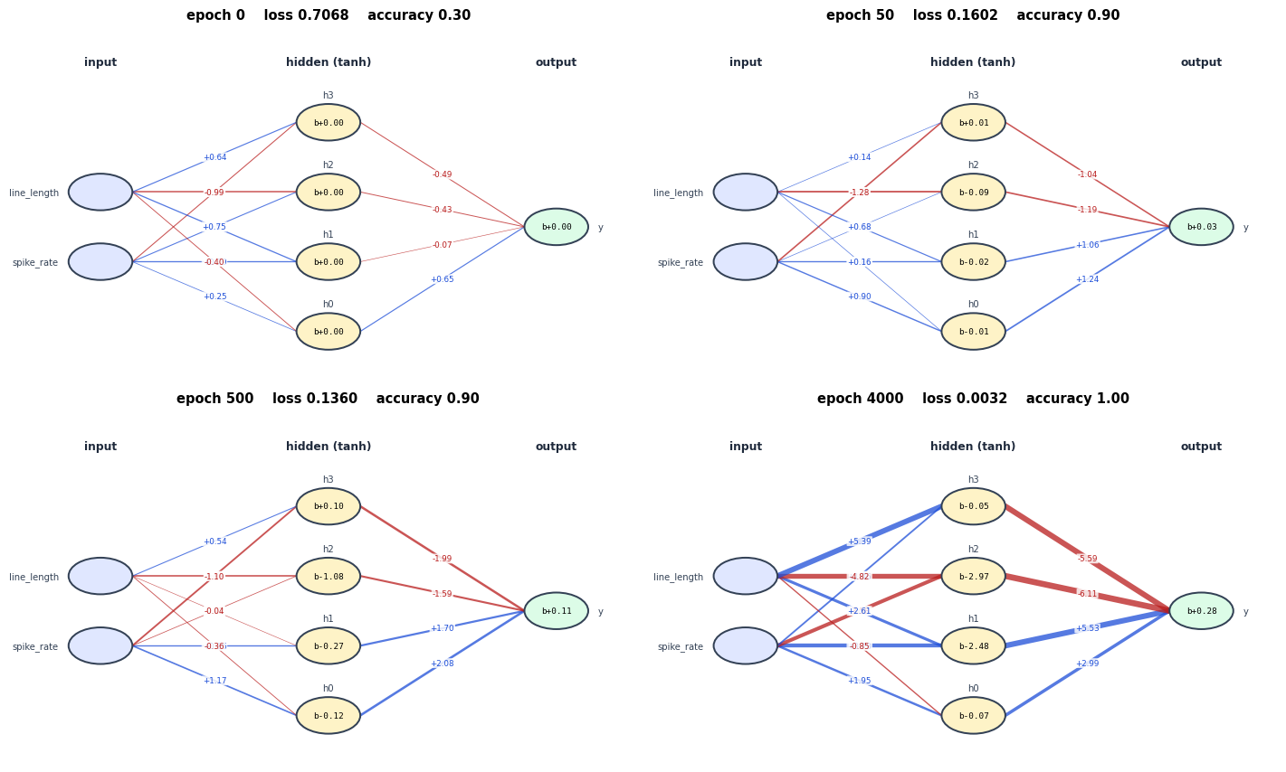
   edge width = |weight|,  blue = positive,  red = negative
1. The Data and the Architecture
The same 20 EEG epochs. A deliberately tiny network so every matrix fits on the page:
$$\underbrace{\mathbf{x}}_{2} \;\xrightarrow{W_1, \mathbf{b}_1}\; \underbrace{\mathbf{z}_1 \to \mathbf{a}_1}_{4 \text{ hidden, tanh}} \;\xrightarrow{W_2, \mathbf{b}_2}\; \underbrace{z_2 \to \hat{y}}_{1 \text{ output, sigmoid}}$$
Parameter count: $W_1$ is $2\times4 = 8$, $\mathbf{b}_1$ is 4, $W_2$ is $4\times1 = 4$, $\mathbf{b}_2$ is 1 — 17 numbers in total.
20 epochs x 2 features, classes [10, 10]

    id   spike_rate   line_length   class         label
-------------------------------------------------------
  ep00          1.0          12.0       0    no seizure
  ep01          1.6          15.0       0    no seizure
  ep02          0.7          11.0       0    no seizure
  ep03          2.1          18.0       0    no seizure
  ep04          1.3          14.0       0    no seizure
  ep05          2.6          21.0       0    no seizure
  ep06          0.9          16.0       0    no seizure
  ep07          1.9          13.0       0    no seizure
  ep08          3.1          24.0       0    no seizure
  ep09          4.4          33.0       0    no seizure
  ep10          6.2          41.0       1       seizure
  ep11          7.1          47.0       1       seizure
  ep12          5.4          38.0       1       seizure
  ep13          8.0          52.0       1       seizure
  ep14          6.7          44.0       1       seizure
  ep15          5.9          49.0       1       seizure
  ep16          7.6          39.0       1       seizure
  ep17          6.0          35.0       1       seizure
  ep18          3.6          27.0       1       seizure
  ep19          8.3          46.0       1       seizure
-------------------------------------------------------

feature means : [ 4.22 29.75]
feature stds  : [ 2.564 13.794]

Note the scales: line_length spans ~41 while spike_rate spans ~8.
Any algorithm that measures DISTANCE will be dominated by the larger one
unless the features are scaled - that matters for KNN and SVM below.
architecture: 2 -> 4 (tanh) -> 1 (sigmoid)
parameters: W1 (2, 4) + b1 (1, 4) + W2 (4, 1) + b2 (1, 1) = 17

W1 (initial) (2, 4) =
                     h0        h1        h2        h3
   spike_rate |   +0.250    +0.794    +0.551    -0.550
   line_length |   -0.400    +0.747    -0.989    +0.642

W2^T (initial) (1, 4) =
                     h0        h1        h2        h3
          out |   +0.651    -0.070    -0.432    -0.485

Xavier init draws from U(-a, a) with a = sqrt(6/(fan_in+fan_out)):
   layer 1: a = sqrt(6/(2+4)) = 1.000000
   layer 2: a = sqrt(6/(4+1)) = 1.095445

Biases start at zero; weights must NOT, or every hidden unit would compute
the same thing forever and the layer would be worth one unit.
2. The Forward Pass
$$\mathbf{z}_1 = XW_1 + \mathbf{b}_1 \qquad \mathbf{a}_1 = \tanh(\mathbf{z}_1)$$ $$z_2 = \mathbf{a}_1W_2 + b_2 \qquad \hat{y} = \sigma(z_2)$$
and the loss is binary cross-entropy, the same one derived in the Logistic Regression walkthrough:
$$\mathcal{L} = -\frac{1}{n}\sum_i\big[y_i\log\hat{y}_i + (1-y_i)\log(1-\hat{y}_i)\big]$$
STEP 1 : z1 = X W1 + b1
==============================================================================
==============================================================================
  X (first 6 rows) (6, 2)   @   W1 (2, 4)   =   X W1 (6, 4)
==============================================================================
  shape rule: (6 x 2) @ (2 x 4) -> (6 x 4)   inner dim 2 cancels
  (20,2) @ (2,4) -> (20,4)
==============================================================================

X (first 6 rows) (6, 2) =
         ep00 |   -1.256    -1.287
         ep01 |   -1.022    -1.069
         ep02 |   -1.373    -1.359
         ep03 |   -0.827    -0.852
         ep04 |   -1.139    -1.142
         ep05 |   -0.632    -0.634

W1 (2, 4) =
            0 |   +0.250    +0.794    +0.551    -0.550
            1 |   -0.400    +0.747    -0.989    +0.642

X W1 (6, 4) =
         ep00 |   +0.200    -1.959    +0.581    -0.136
         ep01 |   +0.172    -1.611    +0.495    -0.125
         ep02 |   +0.200    -2.106    +0.588    -0.119
         ep03 |   +0.134    -1.293    +0.387    -0.093
         ep04 |   +0.171    -1.758    +0.502    -0.108
         ep05 |   +0.095    -0.976    +0.279    -0.060

  worked element  X W1[0,0]  =  row 0 of X (first 6 rows)  .  column 0 of W1
      row 0 of X (first 6 rows) = [-1.256  -1.2867]
      col 0 of W1 = [ 0.2502 -0.3997]
      (-1.2560)*(+0.2502) + (-1.2867)*(-0.3997)
      = +0.200033   |  from array: +0.200033   |  MATCH: True

   then add b1 = [0. 0. 0. 0.] to every row


STEP 2 : a1 = tanh(z1)
==============================================================================
z1 (first 6) (6, 4) =
                     h0        h1        h2        h3
         ep00 |   +0.200    -1.959    +0.581    -0.136
         ep01 |   +0.172    -1.611    +0.495    -0.125
         ep02 |   +0.200    -2.106    +0.588    -0.119
         ep03 |   +0.134    -1.293    +0.387    -0.093
         ep04 |   +0.171    -1.758    +0.502    -0.108
         ep05 |   +0.095    -0.976    +0.279    -0.060

a1 = tanh(z1) (6, 4) =
                     h0        h1        h2        h3
         ep00 |   +0.197    -0.961    +0.523    -0.136
         ep01 |   +0.170    -0.923    +0.458    -0.125
         ep02 |   +0.197    -0.971    +0.528    -0.118
         ep03 |   +0.133    -0.860    +0.369    -0.093
         ep04 |   +0.170    -0.942    +0.463    -0.107
         ep05 |   +0.095    -0.751    +0.272    -0.060

   tanh squashes into (-1, 1): a1 range [-0.9708, +0.9829]
   worked element a1[0,0] = tanh(+0.200033) = +0.197407   MATCH: True


STEP 3 : z2 = a1 W2 + b2,   y_hat = sigmoid(z2)
==============================================================================
==============================================================================
  a1 (first 6) (6, 4)   @   W2 (4, 1)   =   a1 W2 (6, 1)
==============================================================================
  shape rule: (6 x 4) @ (4 x 1) -> (6 x 1)   inner dim 4 cancels
==============================================================================

a1 (first 6) (6, 4) =
         ep00 |   +0.197    -0.961    +0.523    -0.136
         ep01 |   +0.170    -0.923    +0.458    -0.125
         ep02 |   +0.197    -0.971    +0.528    -0.118
         ep03 |   +0.133    -0.860    +0.369    -0.093
         ep04 |   +0.170    -0.942    +0.463    -0.107
         ep05 |   +0.095    -0.751    +0.272    -0.060

W2 (4, 1) =
            0 |   +0.651
            1 |   -0.070
            2 |   -0.432
            3 |   -0.485

a1 W2 (6, 1) =
         ep00 |   +0.036
         ep01 |   +0.038
         ep02 |   +0.026
         ep03 |   +0.033
         ep04 |   +0.029
         ep05 |   +0.026

  worked element  a1 W2[0,0]  =  row 0 of a1 (first 6)  .  column 0 of W2
      row 0 of a1 (first 6) = [ 0.1974 -0.961   0.5232 -0.1356]
      col 0 of W2 = [ 0.6508 -0.0703 -0.4315 -0.4854]
      (+0.1974)*(+0.6508) + (-0.9610)*(-0.0703) + (+0.5232)*(-0.4315) + (-0.1356)*(-0.4854)
      = +0.036043   |  from array: +0.036043   |  MATCH: True

   y_hat[0] = sigmoid(+0.036043) = 0.509010

loss at initialisation = 0.706776
   (a model predicting 0.5 for everything would score 0.693147)
3. Backpropagation
The derivation is the chain rule applied layer by layer, working backwards. Two facts make it short.
Fact 1 — the output layer collapses. Sigmoid with cross-entropy gives exactly the same cancellation as in logistic regression:
$$\frac{\partial \mathcal{L}}{\partial z_2} = \hat{y} - y \;\equiv\; \delta_2$$
Fact 2 — tanh has a cheap derivative. $\tanh'(z) = 1 - \tanh^2(z) = 1 - a_1^2$, so the forward activations are reused rather than recomputed.
Propagating $\delta_2$ backwards:
$$\boxed{\;\delta_2 = \hat{y}-y\;} \qquad \frac{\partial\mathcal{L}}{\partial W_2} = \frac{1}{n}\mathbf{a}_1^\top\delta_2 \qquad \frac{\partial\mathcal{L}}{\partial b_2} = \frac{1}{n}\sum_i \delta_2$$
$$\boxed{\;\delta_1 = (\delta_2 W_2^\top)\odot(1 - \mathbf{a}_1^2)\;} \qquad \frac{\partial\mathcal{L}}{\partial W_1} = \frac{1}{n}X^\top\delta_1 \qquad \frac{\partial\mathcal{L}}{\partial b_1} = \frac{1}{n}\sum_i \delta_1$$
Read $\delta$ as "how much this pre-activation is to blame". The whole algorithm is: compute blame at the output, pass it back through $W^\top$, scale it by the local derivative, repeat.
delta_2 = (y_hat - y) / n     'blame' at the output

    id       y_hat     y    y_hat - y      delta_2
--------------------------------------------------
  ep00    0.509010     0     0.509010     0.025450
  ep01    0.509614     0     0.509614     0.025481
  ep02    0.506454     0     0.506454     0.025323
  ep03    0.508158     0     0.508158     0.025408
  ep04    0.507163     0     0.507163     0.025358
  ep05    0.506610     0     0.506610     0.025331
  ep06    0.491352     0     0.491352     0.024568
  ep07    0.525498     0     0.525498     0.026275
   ...
--------------------------------------------------


delta_1 = (delta_2 W2^T) * (1 - a1^2)     blame pushed back one layer

   step a: delta_2 @ W2^T  -> distributes blame by connection strength
delta_2 @ W2^T (5, 4) =
                     h0        h1        h2        h3
         ep00 |  +0.0165644   -0.0017879   -0.0109828   -0.0123548
         ep01 |  +0.0165840   -0.0017900   -0.0109958   -0.0123695
         ep02 |  +0.0164812   -0.0017789   -0.0109276   -0.0122928
         ep03 |  +0.0165366   -0.0017849   -0.0109644   -0.0123341
         ep04 |  +0.0165043   -0.0017814   -0.0109429   -0.0123100

   step b: multiply by the LOCAL derivative 1 - a1^2
1 - a1^2  (tanh') (5, 4) =
                     h0        h1        h2        h3
         ep00 |  +0.9610305   +0.0764336   +0.7263055   +0.9816224
         ep01 |  +0.9710997   +0.1475768   +0.7904145   +0.9844613
         ep02 |  +0.9611457   +0.0575203   +0.7208205   +0.9860496
         ep03 |  +0.9823761   +0.2604145   +0.8640866   +0.9914426
         ep04 |  +0.9712000   +0.1121413   +0.7851823   +0.9885178

delta_1 (5, 4) =
                     h0        h1        h2        h3
         ep00 |  +0.0159189   -0.0001367   -0.0079768   -0.0121278
         ep01 |  +0.0161047   -0.0002642   -0.0086912   -0.0121773
         ep02 |  +0.0158408   -0.0001023   -0.0078768   -0.0121213
         ep03 |  +0.0162452   -0.0004648   -0.0094742   -0.0122286
         ep04 |  +0.0160290   -0.0001998   -0.0085922   -0.0121687

   worked element delta_1[0,0]:
      = (+0.01656436) * (1 - (+0.197407)^2)
      = (+0.01656436) * (+0.96103052)
      = +0.0159188542
      from the array: +0.0159188542   MATCH: True


gradients

dL/dW1 (2, 4) =
                     h0        h1        h2        h3
   spike_rate |  -0.28078093   +0.00498967   +0.15223398   +0.20902192
   line_length |  -0.27837215   +0.00475220   +0.14475122   +0.20697491

dL/dW2^T (1, 4) =
                     h0        h1        h2        h3
          out |  +0.06544873   -0.38496087   +0.17347403   -0.04000014

dL/db1 = [ 0.0013  0.     -0.0021 -0.0038]
dL/db2 = [-0.0006]
4. Gradient Checking
An analytic gradient that is subtly wrong will still train — badly, and without any error message. The only reliable defence is to compare against a numerical estimate:
$$\frac{\partial\mathcal{L}}{\partial\theta} \approx \frac{\mathcal{L}(\theta+\epsilon) - \mathcal{L}(\theta-\epsilon)}{2\epsilon}$$
The central difference is used rather than the forward one because its error is $O(\epsilon^2)$ instead of $O(\epsilon)$.
This is the single most valuable debugging technique for hand-written networks, so all 17 parameters are checked below.
parameter    analytic (backprop)         numerical    rel. error
--------------------------------------------------------------------
    W1[0, 0]        -0.280780929775   -0.280780929784      1.69e-11
    W1[0, 1]         0.004989666683    0.004989666624      5.89e-09
    W1[0, 2]         0.152233975257    0.152233975370      3.72e-10
    W1[0, 3]         0.209021919936    0.209021919995      1.40e-10
    W1[1, 0]        -0.278372153082   -0.278372153051      5.55e-11
    W1[1, 1]         0.004752195135    0.004752195137      2.87e-10
    W1[1, 2]         0.144751218823    0.144751218789      1.17e-10
    W1[1, 3]         0.206974908490    0.206974908545      1.33e-10
    b1[0, 0]         0.001278761544    0.001278761486      2.28e-08
    b1[0, 1]         0.000010652309    0.000010652257      2.45e-06
    b1[0, 2]        -0.002109805294   -0.002109805275      4.49e-09
    b1[0, 3]        -0.003777413754   -0.003777413771      2.17e-09
    W2[0, 0]         0.065448733576    0.065448733544      2.43e-10
    W2[1, 0]        -0.384960871338   -0.384960871347      1.18e-11
    W2[2, 0]         0.173474031757    0.173474031806      1.40e-10
    W2[3, 0]        -0.040000139442   -0.040000139423      2.37e-10
    b2[0, 0]        -0.000618626289   -0.000618626317      2.28e-08
--------------------------------------------------------------------

parameters checked : 17
max relative error : 2.451e-06
overall relative error (norm form): 1.388e-10

rule of thumb: below 1e-7 the gradient is correct, above 1e-4 it is not.
verdict: CORRECT
What a broken gradient looks like
To show the check actually has teeth, here is the same test with one deliberately introduced bug: forgetting the $(1 - a_1^2)$ factor in $\delta_1$ — a genuinely common slip.
parameter      buggy gradient         numerical    rel. error
----------------------------------------------------------------
    W1[0, 0]       -0.2902986242     -0.2807809298      1.67e-02  <-- WRONG
    W1[0, 1]        0.0313342208      0.0049896666      7.25e-01  <-- WRONG
    W1[0, 2]        0.1924782895      0.1522339754      1.17e-01  <-- WRONG
    W1[0, 3]        0.2165242658      0.2090219200      1.76e-02  <-- WRONG
    W1[1, 0]       -0.2903705458     -0.2783721531      2.11e-02  <-- WRONG
    W1[1, 1]        0.0313419839      0.0047521951      7.37e-01  <-- WRONG
    W1[1, 2]        0.1925259761      0.1447512188      1.42e-01  <-- WRONG
    W1[1, 3]        0.2165779098      0.2069749085      2.27e-02  <-- WRONG
         ...
----------------------------------------------------------------

overall relative error, correct version : 1.388e-10  -> passes
overall relative error, buggy version   : 5.362e-02  -> fails

The buggy version is off by 4e+08x. Note that it would
still 'train' - the loss would go down - just to a worse place, silently.
5. Training
$$\theta \leftarrow \theta - \eta\,\frac{\partial\mathcal{L}}{\partial\theta}$$
Full-batch gradient descent: forward, backward, step, repeat.
training, full batch, eta = 0.5

   epoch     0   loss 0.706776   accuracy 0.3000
   epoch   500   loss 0.136036   accuracy 0.9000
   epoch  1000   loss 0.123009   accuracy 0.9000
   epoch  1500   loss 0.083704   accuracy 0.9500
   epoch  2000   loss 0.022045   accuracy 1.0000
   epoch  2500   loss 0.009480   accuracy 1.0000
   epoch  3000   loss 0.005833   accuracy 1.0000
   epoch  3500   loss 0.004168   accuracy 1.0000
   epoch  4000   loss 0.003226   accuracy 1.0000
The network, drawn — and what learning does to it
Below is the actual network. Every circle is a neuron, every line a weight:
- line thickness = $\lvert w \rvert$, how strongly that connection matters
- blue = positive weight, red = negative
- the number inside each hidden/output circle is its bias
Watching the same diagram at four points during training is the clearest picture of what "learning" means: the structure never changes, only the numbers on the edges.
how the 17 numbers move

  epoch       loss     ||W1||     ||W2||    max |w|   accuracy
------------------------------------------------------------
      0    0.70678     1.8465     0.9222     0.9895     0.3000
     50    0.16023     2.2045     2.2738     1.2835     0.9000
    500    0.13604     2.3822     3.7038     2.0816     0.9000
   4000    0.00323     9.6237    10.3979     6.1111     1.0000
------------------------------------------------------------

At epoch 0 the edges are thin and evenly random - the network has no
opinion. As training proceeds some connections thicken into the ones that
carry the decision, and others fade toward zero. Nothing is added or
removed; the same 17 numbers simply take on useful values.
One epoch, every number
The same loop as the Linear Regression walkthrough — predict, measure error, get the gradient, step — but now with two layers. Three epochs are traced in full, showing every weight before and after.
==============================================================================
  EPOCH 1        loss = 0.706776
==============================================================================

FORWARD - what the network currently predicts (first 5 of 20)

    id      a1[0]      a1[1]      a1[2]      a1[3]      y_hat     y      error
--------------------------------------------------------------------------
  ep00    0.19741   -0.96102    0.52316   -0.13556    0.50901     0    0.50901
  ep01    0.17000   -0.92327    0.45781   -0.12465    0.50961     0    0.50961
  ep02    0.19711   -0.97081    0.52837   -0.11811    0.50645     0    0.50645
  ep03    0.13275   -0.85999    0.36866   -0.09251    0.50816     0    0.50816
  ep04    0.16971   -0.94226    0.46348   -0.10716    0.50716     0    0.50716
--------------------------------------------------------------------------

BACKWARD - blame, layer by layer

   delta_2 (output)  : mean -0.000031,  largest |.| 0.027665
   delta_1 (hidden)  : h0=+0.000064  h1=+0.000001  h2=-0.000105  h3=-0.000189

GRADIENTS

                         h0           h1           h2           h3
--------------------------------------------------------------
   dL/dW1[spike_]   -0.2807809    0.0049897    0.1522340    0.2090219
   dL/dW1[line_l]   -0.2783722    0.0047522    0.1447512    0.2069749
   dL/db1            0.0012788    0.0000107   -0.0021098   -0.0037774
   dL/dW2            0.0654487   -0.3849609    0.1734740   -0.0400001
   dL/db2           -0.0006186
--------------------------------------------------------------

UPDATE   w <- w - 0.5 * gradient

          weight       before    - eta*grad        after
--------------------------------------------------------
     W1[spik,h0]     0.250191     0.1403905     0.390581
     W1[spik,h1]     0.794428    -0.0024948     0.791933
     W1[spik,h2]     0.551371    -0.0761170     0.475254
     W1[spik,h3]    -0.549586    -0.1045110    -0.654097
     W1[line,h0]    -0.399667     0.1391861    -0.260481
     W1[line,h1]     0.747107    -0.0023761     0.744731
     W1[line,h2]    -0.989469    -0.0723756    -1.061845
     W1[line,h3]     0.642457    -0.1034875     0.538969
        W2[h0,y]     0.650847    -0.0327244     0.618122
        W2[h1,y]    -0.070251     0.1924804     0.122229
        W2[h2,y]    -0.431534    -0.0867370    -0.518271
        W2[h3,y]    -0.485445     0.0200001    -0.465445
              b2     0.000000     0.0003093     0.000309
--------------------------------------------------------

   loss: 0.706776  ->  0.505315

==============================================================================
  EPOCH 2        loss = 0.505315
==============================================================================

FORWARD - what the network currently predicts (first 5 of 20)

    id      a1[0]      a1[1]      a1[2]      a1[3]      y_hat     y      error
--------------------------------------------------------------------------
  ep00   -0.15478   -0.96055    0.64720    0.12919    0.35244     0    0.35244
  ep01   -0.12068   -0.92251    0.57218    0.09377    0.37116     0    0.37116
  ep02   -0.18084   -0.97043    0.65944    0.16584    0.34320     0    0.34320
  ep03   -0.10140   -0.85892    0.47191    0.08350    0.38917     0    0.38917
  ep04   -0.14702   -0.94164    0.58638    0.13076    0.36114     0    0.36114
--------------------------------------------------------------------------

BACKWARD - blame, layer by layer

   delta_2 (output)  : mean -0.000117,  largest |.| 0.026764
   delta_1 (hidden)  : h0=-0.000004  h1=-0.000002  h2=+0.000041  h3=-0.000099

GRADIENTS

                         h0           h1           h2           h3
--------------------------------------------------------------
   dL/dW1[spike_]   -0.1929496   -0.0065111    0.1153155    0.1429465
   dL/dW1[line_l]   -0.1937146   -0.0060672    0.1072491    0.1438504
   dL/db1           -0.0000818   -0.0000473    0.0008212   -0.0019854
   dL/dW2           -0.0415299   -0.2798715    0.1590587    0.0364284
   dL/db2           -0.0023352
--------------------------------------------------------------

UPDATE   w <- w - 0.5 * gradient

          weight       before    - eta*grad        after
--------------------------------------------------------
     W1[spik,h0]     0.390581     0.0964748     0.487056
     W1[spik,h1]     0.791933     0.0032556     0.795188
     W1[spik,h2]     0.475254    -0.0576578     0.417597
     W1[spik,h3]    -0.654097    -0.0714732    -0.725570
     W1[line,h0]    -0.260481     0.0968573    -0.163624
     W1[line,h1]     0.744731     0.0030336     0.747764
     W1[line,h2]    -1.061845    -0.0536246    -1.115470
     W1[line,h3]     0.538969    -0.0719252     0.467044
        W2[h0,y]     0.618122     0.0207649     0.638887
        W2[h1,y]     0.122229     0.1399358     0.262165
        W2[h2,y]    -0.518271    -0.0795293    -0.597801
        W2[h3,y]    -0.465445    -0.0182142    -0.483659
              b2     0.000309     0.0011676     0.001477
--------------------------------------------------------

   loss: 0.505315  ->  0.396453

==============================================================================
  EPOCH 3        loss = 0.396453
==============================================================================

FORWARD - what the network currently predicts (first 5 of 20)

    id      a1[0]      a1[1]      a1[2]      a1[3]      y_hat     y      error
--------------------------------------------------------------------------
  ep00   -0.38148   -0.96116    0.72184    0.30337    0.25493     0    0.25493
  ep01   -0.31257   -0.92348    0.64496    0.24020    0.28049     0    0.28049
  ep02   -0.41937   -0.97092    0.73681    0.34897    0.24412     0    0.24412
  ep03   -0.25802   -0.86030    0.54093    0.20222    0.30787     0    0.30787
  ep04   -0.35270   -0.94244    0.66326    0.28768    0.26765     0    0.26765
--------------------------------------------------------------------------

BACKWARD - blame, layer by layer

   delta_2 (output)  : mean -0.000149,  largest |.| 0.028147
   delta_1 (hidden)  : h0=-0.000041  h1=-0.000005  h2=+0.000121  h3=-0.000037

GRADIENTS

                         h0           h1           h2           h3
--------------------------------------------------------------
   dL/dW1[spike_]   -0.1351589   -0.0105975    0.0892332    0.1047640
   dL/dW1[line_l]   -0.1363528   -0.0095995    0.0812392    0.1063079
   dL/db1           -0.0008293   -0.0000917    0.0024242   -0.0007451
   dL/dW2           -0.0750317   -0.2115924    0.1357589    0.0602998
   dL/db2           -0.0029788
--------------------------------------------------------------

UPDATE   w <- w - 0.5 * gradient

          weight       before    - eta*grad        after
--------------------------------------------------------
     W1[spik,h0]     0.487056     0.0675795     0.554636
     W1[spik,h1]     0.795188     0.0052988     0.800487
     W1[spik,h2]     0.417597    -0.0446166     0.372980
     W1[spik,h3]    -0.725570    -0.0523820    -0.777952
     W1[line,h0]    -0.163624     0.0681764    -0.095448
     W1[line,h1]     0.747764     0.0047997     0.752564
     W1[line,h2]    -1.115470    -0.0406196    -1.156089
     W1[line,h3]     0.467044    -0.0531539     0.413890
        W2[h0,y]     0.638887     0.0375159     0.676403
        W2[h1,y]     0.262165     0.1057962     0.367961
        W2[h2,y]    -0.597801    -0.0678795    -0.665680
        W2[h3,y]    -0.483659    -0.0301499    -0.513809
              b2     0.001477     0.0014894     0.002966
--------------------------------------------------------

   loss: 0.396453  ->  0.330778
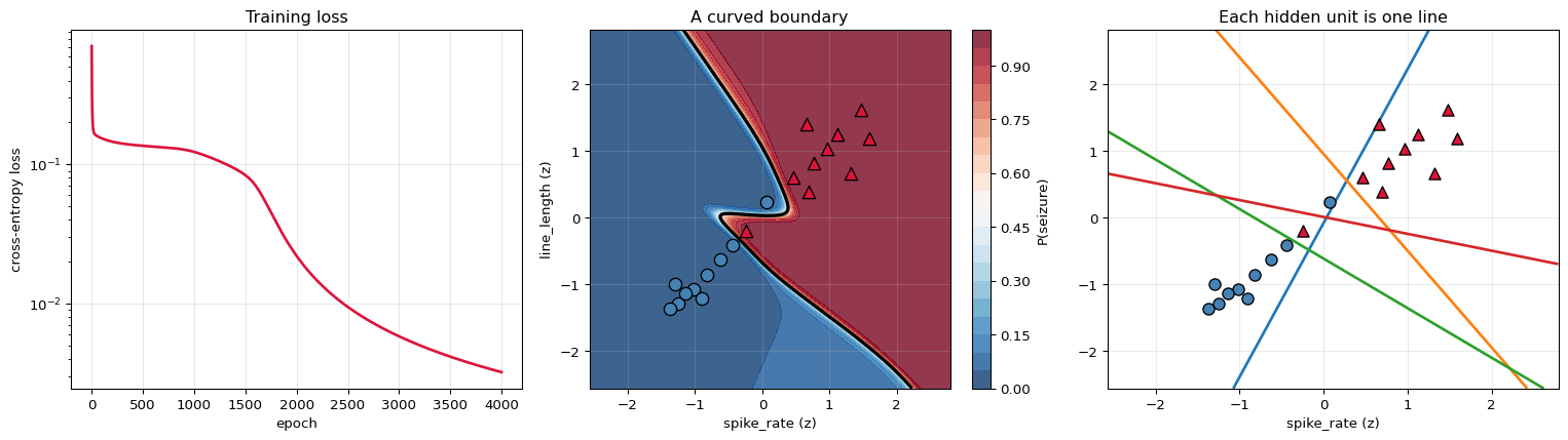
The boundary forming, epoch by epoch
The same training run seen from the outside: what the network actually predicts across the whole feature space as its weights change.
epoch       loss   accuracy                                  what changed
----------------------------------------------------------------------------
      0    0.70678     0.3000           random weights, no structure at all
     20    0.17085     0.9000                  a rough linear split appears
     50    0.16023     0.9000                            the split sharpens
    150    0.14905     0.9000                   the boundary starts to bend
    600    0.13429     0.9000         curvature captures the awkward epochs
   4000    0.00323     1.0000                                     converged
----------------------------------------------------------------------------

final loss     : 0.003226
final accuracy : 1.0000  (20/20)
misclassified  : none

Logistic regression got 18/20 on this data and could not do better -
its boundary is a straight line. The hidden layer removes that limit.
Right panel: each coloured line is where one hidden unit switches sign -
each is still LINEAR. The output layer combines these four half-planes,
and the tanh between them is what lets the combination bend.
Why the non-linearity is essential
Replace $\tanh$ with the identity and the network becomes a product of matrices — an expensive way to write logistic regression. The comparison below makes the collapse concrete.
model        loss   accuracy
----------------------------------------------------------
              2-layer, tanh hidden    0.003226     1.0000
         2-layer, NO non-linearity    0.132144     0.9000
         plain logistic regression    0.132145     0.9000
----------------------------------------------------------

the linear network's effective single weight vector W1 @ W2:
   [ 8.8381 -2.9434]   (bias +0.660633)
   direction, normalised : [ 0.9488 -0.316 ]
   logistic regression   : [ 0.9482 -0.3177]
   cosine similarity     : 0.99999834

The 17-parameter linear network found the SAME direction as the
3-parameter logistic regression, because that is all it can express.
Two linear layers are one linear layer.
6. Activations and Vanishing Gradients
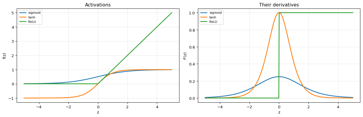
$\delta$ is multiplied by the activation's derivative at every layer. If that derivative is habitually smaller than 1, the product shrinks geometrically with depth — the vanishing gradient problem, and the reason deep networks were impractical before ReLU.
| Activation | $f(z)$ | $f'(z)$ | max $f'$ |
|---|---|---|---|
| Sigmoid | $1/(1+e^{-z})$ | $f(1-f)$ | 0.25 |
| Tanh | $\tanh z$ | $1 - f^2$ | 1.0 |
| ReLU | $\max(0,z)$ | $0$ or $1$ | 1.0 |
what happens to a gradient passed back through L layers

 layers         sigmoid            tanh            ReLU
--------------------------------------------------------
      1       2.500e-01       9.998e-01       1.000e+00
      5       9.764e-04       9.992e-01       1.000e+00
     10       9.533e-07       9.984e-01       1.000e+00
     25       8.873e-16       9.961e-01       1.000e+00
     50       7.873e-31       9.922e-01       1.000e+00
--------------------------------------------------------

With sigmoid the BEST case is 0.25 per layer, so after 25 layers the
gradient is ~1e-15 - numerically zero. Early layers stop learning.
tanh and ReLU have a maximum derivative of 1, which is why they replaced it.


same network, three activations, 2000 epochs each:

  activation    final loss   accuracy
--------------------------------------
        tanh      0.022045     1.0000
     sigmoid      0.137789     0.9000
        ReLU      0.115094     0.9500
--------------------------------------
7. Capacity
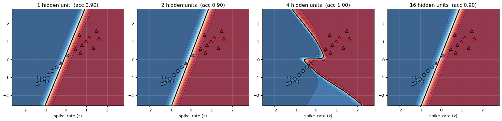
The universal approximation theorem says one hidden layer with enough units can approximate any continuous function to arbitrary accuracy. It says nothing about how many units, or whether gradient descent will find them — and it comes with the usual price: enough capacity to fit anything includes enough capacity to fit noise.
hidden units   parameters    final loss   train acc
----------------------------------------------------
            1            5      0.135725      0.9000
            2            9      0.134148      0.9000
            4           17      0.005833      1.0000
            8           33      0.133313      0.9000
           16           65      0.133089      0.9000
           32          129      0.132797      0.9000
----------------------------------------------------

20 training points and up to 129 parameters - far more knobs
than data. On a real problem that gap is where overfitting lives; here it
is only being used to show the capacity dial working.
One hidden unit can only produce a straight boundary - it is logistic
regression again. Two can bend it. Sixteen wraps tightly around the
individual awkward points, which is memorisation, not understanding.
8. Checking Against scikit-learn
MLPClassifier will not reproduce our exact weights — different initialisation, a
different optimiser, and its own regularisation. What can be checked is that the same
architecture reaches the same quality, and that our forward pass reproduces sklearn's
outputs when handed sklearn's own trained weights.
model   accuracy        loss
----------------------------------------------------
         ours (hand-written)     1.0000    0.003226
       sklearn MLPClassifier     1.0000    0.000027
----------------------------------------------------

now run OUR forward pass using SKLEARN's trained weights:

   W1 (2, 4), b1 (4,), W2 (4, 1), b2 (1,)

    id     our forward    sklearn proba        diff
----------------------------------------------------
  ep00    0.0000020880     0.0000020880    0.00e+00
  ep01    0.0000028418     0.0000028418    0.00e+00
  ep02    0.0000018323     0.0000018323    0.00e+00
  ep03    0.0000051654     0.0000051654    8.47e-22
  ep04    0.0000020440     0.0000020440    4.24e-22
  ep05    0.0000184342     0.0000184342    3.39e-21
  ep06    0.0000000000     0.0000000000    0.00e+00
  ep07    0.0000082756     0.0000082756    1.69e-21
   ...
----------------------------------------------------

all 20 outputs MATCH: True
max difference: 5.421e-20

That confirms the forward pass is exactly the operation sklearn performs.
The gradient check in section 4 confirms the backward pass. Together they
establish the implementation, without needing identical weights.
9. Summary
| Stage | Formula |
|---|---|
| Forward, layer 1 | $\mathbf{z}_1 = XW_1+\mathbf{b}_1$, $\;\mathbf{a}_1 = \tanh\mathbf{z}_1$ |
| Forward, layer 2 | $z_2 = \mathbf{a}_1W_2+b_2$, $\;\hat{y} = \sigma(z_2)$ |
| Loss | binary cross-entropy |
| Output blame | $\delta_2 = \hat{y}-y$ |
| Hidden blame | $\delta_1 = (\delta_2W_2^\top)\odot(1-\mathbf{a}_1^2)$ |
| Gradients | $\frac{1}{n}\mathbf{a}_1^\top\delta_2$, $\;\frac{1}{n}X^\top\delta_1$ |
| Update | $\theta \leftarrow \theta - \eta\nabla_\theta\mathcal{L}$ |
| Verification | central differences, rel. error $< 10^{-7}$ |
The one idea: backpropagation is the chain rule with the intermediate results kept. A naive approach would recompute the shared prefix for every parameter; backprop computes each $\delta$ once and reuses it, which is what makes the cost of the backward pass roughly equal to the forward pass rather than proportional to the parameter count.
What the non-linearity buys: without it, depth is an illusion — section 5 shows a 17-parameter linear network converging to exactly the direction that 3-parameter logistic regression finds. With it, the same network draws a boundary neither could.
What is deliberately left out: mini-batch SGD and momentum, Adam and adaptive learning rates, dropout, batch normalisation, weight decay, learning-rate schedules, softmax with multiple classes, convolutional and recurrent structure, and automatic differentiation — which is this notebook's backward pass, generalised and generated rather than derived by hand.