🚀 Optimisers: SGD to Adam
The Concepts walkthrough stopped at plain gradient descent:
$$w \leftarrow w - \eta\,\nabla\mathcal{L}$$
Almost nobody uses that. Every training script reaches for Adam, and most people who
type it could not say what it does. This notebook builds up to it in four steps, each one
fixing a specific failure of the one before, with every update computed by hand.
| Optimiser | What it adds | The problem it fixes |
|---|---|---|
| SGD | — | — |
| Momentum | a velocity term | zig-zagging in narrow valleys |
| RMSProp | per-parameter step sizes | parameters on wildly different scales |
| Adam | both, plus bias correction | both, plus a bad start |
The point to hold onto: all four use the identical gradient. They differ only in what they do with it.
Display helpers ready: banner, step, check, expand, show_matrix, show_matmul, show_elementwise.
1. A Loss Surface That Breaks Plain SGD
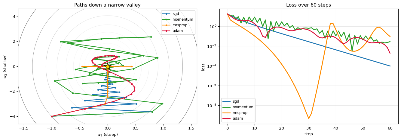
The classic hard case is a narrow valley — steep in one direction, nearly flat in another:
$$\mathcal{L}(w_1, w_2) = \tfrac{1}{2}\big(a\,w_1^2 + b\,w_2^2\big), \qquad a \gg b$$
The gradient is dominated by the steep direction, so descent bounces across the valley while barely advancing along it. The severity is captured by the condition number $\kappa = a/b$: gradient descent needs roughly $O(\kappa)$ steps.
loss(w1, w2) = 0.5 * (20.0*w1^2 + 1.0*w2^2)
minimum at (0, 0), where the loss is 0

curvature along w1 : 20.0
curvature along w2 : 1.0
condition number   : 20

stability limit for plain SGD: eta < 2/20.0 = 0.1000
   -> the STEEP direction caps the step size, but the SHALLOW direction
      is the one that needs large steps. That conflict is the problem.

starting at w = [-1. -4.], loss = 18.0000

 step          w1          w2     grad w1     grad w2        loss
--------------------------------------------------------------
    0   -1.000000   -4.000000    -20.0000     -4.0000   18.000000
    1    0.800000   -3.640000     16.0000     -3.6400   13.024800
    2   -0.640000   -3.312400    -12.8000     -3.3124    9.581997
    3    0.512000   -3.014284     10.2400     -3.0143    7.164394
    4   -0.409600   -2.742998     -8.1920     -2.7430    5.439742
    5    0.327680   -2.496129      6.5536     -2.4961    4.189071
--------------------------------------------------------------

look at w1: it flips sign every single step - the classic zig-zag.
   the gradient in w1 is 20x larger than in w2, so w1 overshoots
   while w2 creeps.

after 6 steps: w2 has moved from -4.0 to -2.2715 - barely
43.2% of the way.
2. Momentum — Remember Where You Were Going
Instead of stepping along the current gradient, accumulate a velocity:
$$\mathbf{v}_t = \beta\,\mathbf{v}_{t-1} + \nabla\mathcal{L} \qquad\qquad \mathbf{w} \leftarrow \mathbf{w} - \eta\,\mathbf{v}_t$$
The physical picture is a ball rolling downhill rather than a walker re-deciding at each step. Two effects follow, and both help:
- Components that keep pointing the same way (the shallow direction) accumulate, so progress accelerates — up to $1/(1-\beta)$ times faster.
- Components that alternate sign (the zig-zag) cancel against their own history.
With $\beta = 0.9$ the effective step along a consistent direction is up to $1/(1-0.9) = 10\times$ larger.
momentum, beta = 0.9, eta = 0.09

 step                  grad             v = b*v + g               w after       loss
----------------------------------------------------------------------------------
    0           [-20.  -4.]  0.9*[0. 0.] + [-20.  -4.]         [ 0.8  -3.64]   18.00000
    1         [16.   -3.64]  0.9*[-20.  -4.] + [16.   -3.64]     [ 0.98   -2.9884]   13.02480
    2     [19.6    -2.9884]  0.9*[-2.   -7.24] + [19.6   -2.988]       [-0.622 -2.133]   14.06927
    3     [-12.44   -2.133]       [  3.58  -10.687]     [-0.9442 -1.1712]    6.14369
    4   [-18.884   -1.1712]     [-15.662  -10.7894]     [ 0.4654 -0.2001]    9.60096
    5     [ 9.3076 -0.2001]       [-4.7882 -9.9106]       [0.8963 0.6918]    2.18581
----------------------------------------------------------------------------------

after 6 steps: loss 8.273173
plain SGD after 6 steps: loss 3.266999

momentum is 0.4x lower

the velocity in the SHALLOW direction, accumulating:

 step    gradient w2    velocity w2   amplification
--------------------------------------------------
    0      -4.000000      -4.000000          1.000x
    1      -3.640000      -7.240000          1.989x
    2      -2.988400      -9.504400          3.180x
    3      -2.133004     -10.686964          5.010x
    4      -1.171177     -10.789445          9.212x
    5      -0.200127      -9.910628         49.522x
    6       0.691829      -8.227736        -11.893x
    7       1.432325      -5.972637         -4.170x
--------------------------------------------------

theoretical ceiling: 1/(1 - 0.9) = 10.0x

Meanwhile in w1 the gradient keeps flipping sign, so the velocity there
partly cancels itself instead of accumulating - exactly the damping we want.
3. RMSProp — A Different Step Size Per Parameter
Momentum still uses one learning rate for every parameter. But in the valley above, $w_1$ needs small steps and $w_2$ needs large ones. RMSProp gives each its own, by tracking a running average of squared gradients and dividing by the root:
$$s_t = \rho\,s_{t-1} + (1-\rho)\,g_t^2 \qquad\qquad w \leftarrow w - \frac{\eta}{\sqrt{s_t} + \epsilon}\,g_t$$
Read $\sqrt{s_t}$ as "how big have this parameter's gradients typically been". Dividing by it normalises the step: a parameter with consistently huge gradients gets a small effective rate, one with tiny gradients gets a large one.
$\epsilon$ (usually $10^{-8}$) exists only to stop division by zero.
RMSProp, rho = 0.9, eta = 0.3

 step                grad           s (avg g^2)           eta/sqrt(s)       loss
------------------------------------------------------------------------------
    0         [-20.  -4.]           [40.   1.6]       [0.0474 0.2372]   18.00000
    1   [-1.0263 -3.0513]     [36.1053  2.3711]       [0.0499 0.1948]    4.68160
    2   [-0.0015 -2.4568]     [32.4948  2.7376]       [0.0526 0.1813]    3.01802
    3   [ 0.0001 -2.0114]     [29.2453  2.8684]       [0.0555 0.1771]    2.02280
    4   [-0.     -1.6551]     [26.3208  2.8555]       [0.0585 0.1775]    1.36965
    5   [ 0.     -1.3612]     [23.6887  2.7552]       [0.0616 0.1807]    0.92650
------------------------------------------------------------------------------

after 6 steps: loss 0.621861

the effective learning rate per parameter, side by side:

   step 0:  |g1| =  20.0000 -> rate 0.04743     |g2| =   4.0000 -> rate 0.23717     ratio 5.00x
   step 1:  |g1| =   1.0263 -> rate 0.04993     |g2| =   3.0513 -> rate 0.19483     ratio 3.90x
   step 2:  |g1| =   0.0015 -> rate 0.05263     |g2| =   2.4568 -> rate 0.18132     ratio 3.45x

The shallow parameter is given a step 3.4x larger. Plain SGD
could never do that - it has only one eta for both.


step 0 written out in full:

   g       = [-20.  -4.]
   g^2     = [400.  16.]
   s = 0.9*[0. 0.] + 0.1*[400.  16.] = [40.   1.6]
   sqrt(s) = [6.3246 1.2649]
   step    = 0.3 / ([6.3246 1.2649] + eps) * [-20.  -4.]
           = [-0.9487 -0.9487]
   w       = [-1. -4.] - [-0.9487 -0.9487] = [-0.0513 -3.0513]
4. Adam — Both, Plus a Fix for the Start
Adam ("adaptive moment estimation") keeps both running averages: the mean of the gradient (like momentum) and the mean of its square (like RMSProp).
$$m_t = \beta_1 m_{t-1} + (1-\beta_1)g_t \qquad\text{(1st moment: direction)}$$ $$v_t = \beta_2 v_{t-1} + (1-\beta_2)g_t^2 \qquad\text{(2nd moment: scale)}$$
Then the part that is usually skipped in explanations. Both start at zero, so early on they are biased toward zero — after one step $m_1 = (1-\beta_1)g_1 = 0.1\,g_1$, ten times too small. Adam divides that bias out:
$$\hat{m}_t = \frac{m_t}{1-\beta_1^{\,t}} \qquad\qquad \hat{v}_t = \frac{v_t}{1-\beta_2^{\,t}}$$
$$w \leftarrow w - \frac{\eta}{\sqrt{\hat{v}_t}+\epsilon}\,\hat{m}_t$$
At $t=1$, $1-\beta_1^1 = 0.1$, so dividing by it multiplies $m_1$ back up by exactly 10 — recovering $g_1$. The correction fades as $\beta^t \to 0$, so it only matters at the start.
Adam, beta1 = 0.9, beta2 = 0.999, eta = 0.3

  t                  g                  m              m_hat              v_hat       loss
--------------------------------------------------------------------------------------------
  1        [-20.  -4.]        [-2.  -0.4]        [-20.  -4.]        [400.  16.]   18.00000
  2      [-14.   -3.7]      [-3.2  -0.73]  [-16.842  -3.842]  [297.949  14.844]   11.74500
  3    [-8.146 -3.401]    [-3.695 -0.997]  [-13.633  -3.679]  [220.673  13.75 ]    7.44165
  4    [-2.639 -3.103]    [-3.589 -1.208]  [-10.436  -3.512]  [167.166  12.719]    4.98898
  5    [ 2.204 -2.808]    [-3.01  -1.368]      [-7.35 -3.34]  [134.639  11.75 ]    4.06319
  6    [ 6.004 -2.515]    [-2.108 -1.482]    [-4.5   -3.164]  [118.167  10.844]    4.06505
--------------------------------------------------------------------------------------------

after 6 steps: loss 4.28135325


step t = 1, in full - and what bias correction does

   g_1     = [-20.  -4.]
   m_1     = 0.9*0 + 0.1*g = [-2.  -0.4]   <- only 10% of the gradient!
   v_1     = 0.999*0 + 0.001*g^2 = [0.4   0.016]

   bias correction divides by (1 - beta^t):
   1 - beta1^1 = 0.1000   ->  m_hat = [-2.  -0.4] / 0.1000 = [-20.  -4.]
   1 - beta2^1 = 0.0010   ->  v_hat = [0.4   0.016] / 0.0010 = [400.  16.]

   m_hat == g_1 exactly? True
   So at t=1 Adam's direction is simply the gradient, as it should be.


how long the correction matters:

    t     1 - b1^t     1 - b2^t    m inflated by    v inflated by
----------------------------------------------------------------
    1     0.100000     0.001000          10.000x        1000.000x
    2     0.190000     0.001999           5.263x         500.250x
    5     0.409510     0.004990           2.442x         200.400x
   10     0.651322     0.009955           1.535x         100.451x
   50     0.994846     0.048794           1.005x          20.494x
  200     1.000000     0.181351           1.000x           5.514x
 1000     1.000000     0.632305           1.000x           1.582x
 5000     1.000000     0.993279           1.000x           1.007x
----------------------------------------------------------------

By t = 50 the first-moment correction is negligible; the second-moment
one (beta2 = 0.999) persists for thousands of steps. Without it, early
updates would be far too large - v_hat too small means dividing by a
too-small number.


with and without bias correction, first 5 steps:

 step    corrected loss    uncorrected loss
--------------------------------------------
    0         18.000000           18.000000
    1         11.745000            4.681601
    2          7.441645            8.846616
    3          4.988979            7.388804
    4          4.063193            1.562467
    5          4.065053            2.813670
--------------------------------------------
5. All Four on the Same Surface
optimiser         loss@5        loss@10        loss@25        loss@60
------------------------------------------------------------------------
         sgd      4.189e+00      1.328e+00      7.178e-02      9.729e-05
    momentum      2.186e+00      8.790e+00      4.341e-01      2.863e-02
     rmsprop      9.265e-01      1.073e-01      7.415e-07      9.548e-02
        adam      4.065e+00      1.910e+00      4.164e-01      1.951e-03
------------------------------------------------------------------------

steps needed to reach loss < 1e-4:

          sgd: 60
     momentum: > 60
      rmsprop: 21
         adam: > 60
SGD zig-zags across the valley. Momentum damps the zig-zag and picks up
speed along it. RMSProp instead rescales each axis so the valley becomes
round. Adam does both, which is why it is the default.
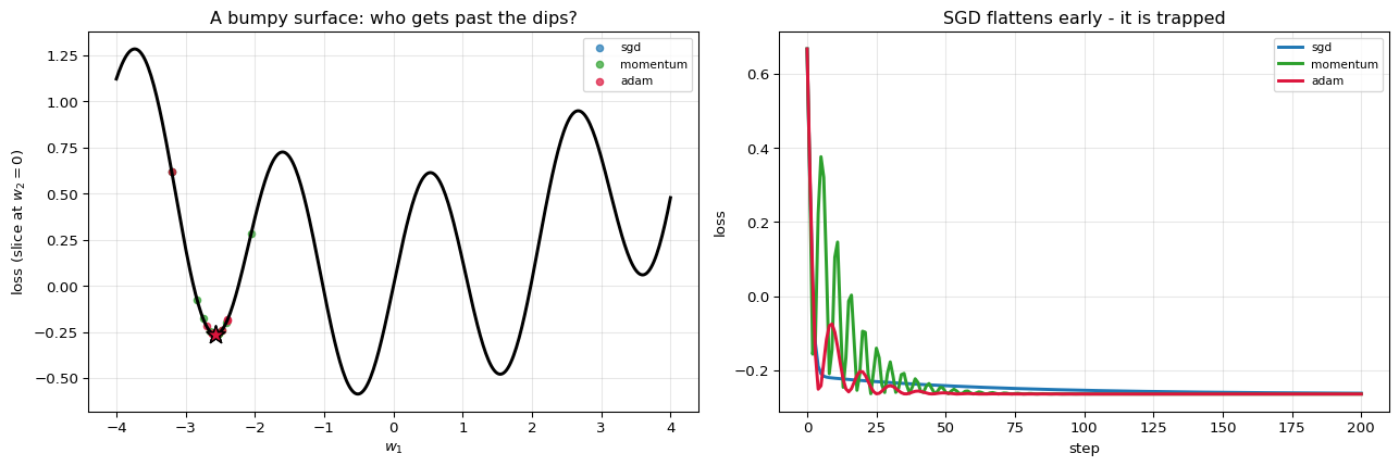
A surface with a local dip
The valley showed scale. This one shows the other thing momentum buys: enough inertia to roll through a small local minimum that would trap plain descent.
optimiser    final w1    final loss                     outcome
------------------------------------------------------------------
         sgd     -2.5702     -0.261535        STUCK in a local dip
    momentum     -2.5701     -0.263547        STUCK in a local dip
        adam     -2.5702     -0.263547        STUCK in a local dip
------------------------------------------------------------------
SGD stops at the first dip it meets, because the gradient there is zero
and it has no memory. Momentum arrives carrying velocity and rolls
through. This is the intuition behind 'momentum escapes local minima' -
though on real high-dimensional surfaces the more important effect is
simply that it damps oscillation and accelerates consistent directions.
6. Checking Against PyTorch
Adam has enough moving parts that an off-by-one in the bias correction is easy and
silent. The check: run our implementation and torch.optim.Adam from identical starting
points and compare the parameter trajectories step by step.
optimiser                 our final w               torch final w    match
------------------------------------------------------------------------------
         sgd           [ 0.0038 -0.3785]           [ 0.0038 -0.3785]     True
    momentum           [-0.1994 -0.2708]           [-0.1994 -0.2708]     True
     rmsprop           [ 0.     -0.0012]           [ 0.     -0.0012]     True
        adam             [0.0737 0.8511]             [0.0737 0.8511]     True
------------------------------------------------------------------------------


Adam trajectory, step by step

 step        ours w1       torch w1        ours w2       torch w2
------------------------------------------------------------------
    0   -1.000000000   -1.000000000   -4.000000000   -4.000000000
    1   -0.700000000   -0.700000000   -3.700000001   -3.700000001
    2   -0.407283850   -0.407283850   -3.400836323   -3.400836323
    3   -0.131961645   -0.131961645   -3.103172802   -3.103172802
    4    0.110193129    0.110193129   -2.807763388   -2.807763388
    5    0.300213834    0.300213834   -2.515460095   -2.515460095
    6    0.424393572    0.424393572   -2.227219885   -2.227219885
    7    0.481489841    0.481489841   -1.944109524   -1.944109524
    8    0.480525501    0.480525501   -1.667307182   -1.667307182
------------------------------------------------------------------

full-trajectory MATCH: True
max difference: 1.110e-16


note on torch's momentum convention:
   ours  : v = beta*v + g   then  w -= eta*v
   torch : identical (this is 'heavy ball', not Nesterov)
   trajectories agree: True

Some papers instead write v = beta*v + (1-beta)*g, which rescales the
effective learning rate by (1-beta). Both appear in the literature, so
a learning rate is only meaningful alongside its momentum convention.
7. Practical Notes
Adam is not always better. For image classification, well-tuned SGD with momentum often generalises better than Adam, even though Adam reaches a lower training loss faster. The adaptive step sizes appear to favour sharper minima. Adam's real strength is that it works acceptably with almost no tuning, which matters when you cannot afford a learning-rate search.
AdamW fixes weight decay. Adding $\lambda\lVert w\rVert^2$ to the loss is not equivalent to shrinking $w$ each step once the update is divided by $\sqrt{\hat{v}}$ — the decay gets scaled by the adaptive term too. AdamW applies the decay separately, and is the correct default for Transformers.
Learning-rate schedules still matter. Adaptive step sizes are not a schedule; warmup and cosine decay remain standard.
effective step size Adam takes, regardless of gradient magnitude

    gradient         m_hat    sqrt(v_hat)    m_hat/sqrt(v_hat)
--------------------------------------------------------------
       1e-04    1.0000e-04     1.0000e-04             1.000000
       1e-02    1.0000e-02     1.0000e-02             1.000000
       1e+00    1.0000e+00     1.0000e+00             1.000000
       1e+02    1.0000e+02     1.0000e+02             1.000000
       1e+04    1.0000e+04     1.0000e+04             1.000000
--------------------------------------------------------------

For a CONSTANT gradient the ratio is 1 whatever its size - so Adam's step
is about eta, regardless of scale. That is the property that makes it
robust to badly scaled problems, and also why its eta means something
different from SGD's (1e-3 is a typical Adam default, vs 1e-1 for SGD).

   optimiser    typical eta    needs tuning?                    common use
--------------------------------------------------------------------------
         SGD    1e-2 - 1e-1            a lot     when you can tune, vision
    Momentum    1e-2 - 1e-1            a lot       SGD's default companion
     RMSProp           1e-3             some              RNNs, older code
        Adam           1e-3           little             almost everything
       AdamW           1e-3           little                  Transformers
--------------------------------------------------------------------------
8. Summary
| Optimiser | Update |
|---|---|
| SGD | $w \leftarrow w - \eta g$ |
| Momentum | $v \leftarrow \beta v + g$; $\;w \leftarrow w - \eta v$ |
| RMSProp | $s \leftarrow \rho s + (1-\rho)g^2$; $\;w \leftarrow w - \frac{\eta}{\sqrt{s}+\epsilon}g$ |
| Adam | $m,v$ as above; $\hat m = \frac{m}{1-\beta_1^t}$, $\hat v = \frac{v}{1-\beta_2^t}$; $\;w \leftarrow w - \frac{\eta}{\sqrt{\hat v}+\epsilon}\hat m$ |
The one idea: the gradient tells you the direction. Everything after SGD is about choosing the step, using information the raw gradient does not contain — its recent history (momentum) and its typical magnitude per parameter (RMSProp).
Why bias correction exists: both moving averages start at zero, so early estimates are biased toward zero. Dividing by $1-\beta^t$ removes exactly that bias, and at $t=1$ recovers the raw gradient. It is three characters of code and easy to omit, and omitting it makes the first few hundred steps wrong.
What is deliberately left out: Nesterov momentum, AdaGrad (RMSProp's ancestor, whose denominator grows without bound so the rate decays to zero), AdaDelta, LAMB and LARS for very large batches, second-order methods (L-BFGS, K-FAC), and learning-rate schedules, which are a separate lever from the optimiser.