🌀 Principal Component Analysis
The KNN walkthrough ended on a problem: in high dimensions every point is roughly the same distance from every other, and distance-based methods stop working. PCA is the standard answer — find a smaller set of directions that keeps most of the information.
The idea can be stated two ways, and they turn out to be the same optimisation:
- Maximise variance. Find the direction along which the data is most spread out, then the best direction orthogonal to that, and so on.
- Minimise reconstruction error. Find the $k$-dimensional subspace whose orthogonal projection loses the least squared distance.
Both lead to the eigenvectors of the covariance matrix:
$$\Sigma = \frac{1}{n-1}X_c^\top X_c, \qquad \Sigma\mathbf{v} = \lambda\mathbf{v}$$
The eigenvector with the largest $\lambda$ is the first principal component, and $\lambda$ is the variance along it. Everything below computes $\Sigma$, its eigenvectors and the projection by hand, shows the SVD route to the same answer, and checks against scikit-learn.
Display helpers ready: banner, step, check, expand, show_matrix, show_matmul, show_elementwise.
1. The Data
The 12 EEG recordings and their three features. These features are strongly correlated — a recording with a high spike rate also tends to have a high line length — which is exactly the redundancy PCA exists to remove.
12 recordings x 3 features

    id      region   line_length    spike_rate           age   y_class    y_reg
-------------------------------------------------------------------------------
 rec00     frontal          12.0           0.5          24.0         0      0.2
 rec01    temporal          15.0           1.2          31.0         0      0.5
 rec02    temporal          42.0           6.8          58.0         1      6.4
 rec03   occipital          38.0           5.1          47.0         1      4.8
 rec04     frontal          11.0           0.3          19.0         0      0.1
 rec05    temporal          55.0           8.2          63.0         1      9.1
 rec06   occipital          40.0           1.9          35.0         1      3.5
 rec07    temporal          47.0           7.4          52.0         1      7.2
 rec08     frontal          14.0           0.8          28.0         0      0.3
 rec09   occipital          51.0           6.1          60.0         1      6.9
 rec10     frontal          45.0           2.4          41.0         0      1.6
 rec11    temporal          35.0           4.7          30.0         1      4.1
-------------------------------------------------------------------------------

class balance: 5 negative, 7 positive
y_reg mean = 3.7250, std = 3.0518
correlation between the raw features

correlation (3, 3) =
             line_lengthspike_rate       age
   line_length |  +1.0000   +0.8509   +0.8806
   spike_rate |  +0.8509   +1.0000   +0.9085
          age |  +0.8806   +0.9085   +1.0000

Every pair is correlated above 0.85.
Three columns, but far less than three dimensions worth of information -
that gap is what PCA measures and removes.
2. Centring (and Scaling)
PCA measures variance about the mean, so the data must be centred first. Without it the first component points at the mean itself rather than at the direction of spread.
Whether to scale as well is a modelling choice, not a technicality:
- Covariance PCA (centre only) — a feature measured in larger numbers gets more say. Appropriate when the units are genuinely comparable.
- Correlation PCA (centre and standardise) — every feature contributes equally.
Here age runs to 63 while spike_rate runs to 8, so unstandardised PCA would be almost
entirely about age. Both are computed below so the difference is visible.
feature means : [33.75    3.7833 40.6667]
feature stds  : [16.2656  2.9167 15.0414]

X centred (12, 3) =
             line_lengthspike_rate       age
        rec00 |  -21.750    -3.283   -16.667
        rec01 |  -18.750    -2.583    -9.667
        rec02 |   +8.250    +3.017   +17.333
        rec03 |   +4.250    +1.317    +6.333
        rec04 |  -22.750    -3.483   -21.667
        rec05 |  +21.250    +4.417   +22.333
        rec06 |   +6.250    -1.883    -5.667
        rec07 |  +13.250    +3.617   +11.333
        rec08 |  -19.750    -2.983   -12.667
        rec09 |  +17.250    +2.317   +19.333
        rec10 |  +11.250    -1.383    +0.333
        rec11 |   +1.250    +0.917   -10.667

column means after centring: [0. 0. 0.]
all zero? True

     feature   variance (raw)   share of total
----------------------------------------------
 line_length         264.5682           53.0%
  spike_rate           8.5070            1.7%
         age         226.2424           45.3%
----------------------------------------------

'line_length' alone accounts for 53.0% of the raw
variance - purely because of its units. That is what standardising fixes.
3. The Covariance Matrix
$$\Sigma_{jk} = \frac{1}{n-1}\sum_{i=1}^{n}(x_{ij}-\bar{x}_j)(x_{ik}-\bar{x}_k) \qquad\Longleftrightarrow\qquad \Sigma = \frac{1}{n-1}X_c^\top X_c$$
The diagonal holds the variances, the off-diagonal the covariances. It is symmetric, which guarantees real eigenvalues and orthogonal eigenvectors — the property the whole method rests on.
==============================================================================
  Xc^T (3, 12)   @   Xc (12, 3)   =   Xc^T Xc (3, 3)
==============================================================================
  shape rule: (3 x 12) @ (12 x 3) -> (3 x 3)   inner dim 12 cancels
  then divide by n-1 = 11
==============================================================================

Xc^T (3, 12) =
            0 |  -21.750   -18.750    +8.250    +4.250   -22.750   +21.250    +6.250   +13.250   -19.750   +17.250   +11.250    +1.250
            1 |   -3.283    -2.583    +3.017    +1.317    -3.483    +4.417    -1.883    +3.617    -2.983    +2.317    -1.383    +0.917
            2 |  -16.667    -9.667   +17.333    +6.333   -21.667   +22.333    -5.667   +11.333   -12.667   +19.333    +0.333   -10.667

Xc (12, 3) =
            0 |  -21.750    -3.283   -16.667
            1 |  -18.750    -2.583    -9.667
            2 |   +8.250    +3.017   +17.333
            3 |   +4.250    +1.317    +6.333
            4 |  -22.750    -3.483   -21.667
            5 |  +21.250    +4.417   +22.333
            6 |   +6.250    -1.883    -5.667
            7 |  +13.250    +3.617   +11.333
            8 |  -19.750    -2.983   -12.667
            9 |  +17.250    +2.317   +19.333
           10 |  +11.250    -1.383    +0.333
           11 |   +1.250    +0.917   -10.667

Xc^T Xc (3, 3) =
            0 | +2910.250  +444.050  +2370.000
            1 | +444.050   +93.577  +438.433
            2 | +2370.000  +438.433  +2488.667

  worked element  Xc^T Xc[0,0]  =  row 0 of Xc^T  .  column 0 of Xc
      row 0 of Xc^T = [-21.75 -18.75   8.25   4.25 -22.75  21.25   6.25  13.25 -19.75  17.25  11.25   1.25]
      col 0 of Xc = [-21.75 -18.75   8.25   4.25 -22.75  21.25   6.25  13.25 -19.75  17.25  11.25   1.25]
      (-21.7500)*(-21.7500) + (-18.7500)*(-18.7500) + (+8.2500)*(+8.2500) + (+4.2500)*(+4.2500) +
      (-22.7500)*(-22.7500) + (+21.2500)*(+21.2500) + (+6.2500)*(+6.2500) + (+13.2500)*(+13.2500) +
      (-19.7500)*(-19.7500) + (+17.2500)*(+17.2500) + (+11.2500)*(+11.2500) + (+1.2500)*(+1.2500)
      = +2910.250000   |  from array: +2910.250000   |  MATCH: True

Sigma = Xc^T Xc / (n-1) (3, 3) =
             line_lengthspike_rate       age
   line_length |   +264.5682     +40.3682    +215.4545
   spike_rate |    +40.3682      +8.5070     +39.8576
          age |   +215.4545     +39.8576    +226.2424

by hand, Sigma[0,1] (covariance of line_length and spike_rate):
   sum of products = (+71.41) + (+48.44) + (+24.89) + (+5.60) + (+79.25) + ...
                   = 444.050000
   / (n-1)         = 444.050000 / 11 = 40.368182
   from the matrix : 40.368182   MATCH: True

symmetric? True
diagonal = per-feature variances? True
trace (total variance) = 499.317576
matches np.cov? True
4. Eigendecomposition
$$\Sigma\mathbf{v} = \lambda\mathbf{v}$$
For each eigenvector $\mathbf{v}$, the variance of the data projected onto it is exactly $\lambda$:
$$\operatorname{Var}(X_c\mathbf{v}) = \mathbf{v}^\top\Sigma\mathbf{v} = \mathbf{v}^\top\lambda\mathbf{v} = \lambda$$
That identity is why "largest eigenvalue" and "direction of greatest variance" are the same thing — and it is verified numerically below.
eigenvalues, largest first

  PC     eigenvalue   variance share    cumulative
--------------------------------------------------
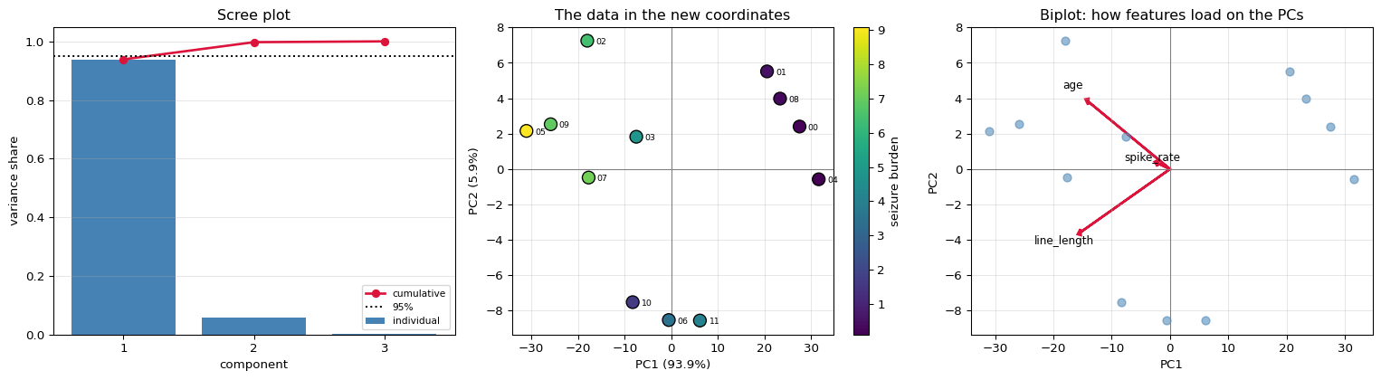
PC 1     468.693715          93.87%       93.87%
PC 2      29.264932           5.86%       99.73%
PC 3       1.358929           0.27%      100.00%
--------------------------------------------------
sum of eigenvalues = 499.317576
trace of Sigma     = 499.317576
MATCH: True

(that equality is not a coincidence - PCA redistributes the same total
 variance across new axes, it does not create or destroy any)

eigenvectors (the principal directions)

components (rows = PC1, PC2, PC3) (3, 3) =
             line_lengthspike_rate       age
          PC1 |  -0.731824   -0.122264   -0.670436
          PC2 |  -0.680432   +0.076208   +0.728838
          PC3 |  +0.038018   -0.989567   +0.138963

verifying Sigma v = lambda v for PC1:

   Sigma @ v1  = [-343.0015  -57.3045 -314.2291]
   lambda * v1 = [-343.0015  -57.3045 -314.2291]
   MATCH: True

orthonormality:
   ||v1|| = 1.0000000000
   v1.v2  = +2.220e-16
   V^T V = I ? True
the key identity: variance along a direction = its eigenvalue

  PC    var of projection     eigenvalue    match
--------------------------------------------------
PC 1         468.69371465   468.69371465     True
PC 2          29.26493224    29.26493224     True
PC 3           1.35892887     1.35892887     True
--------------------------------------------------

and no other direction beats PC1 - testing 20000 random unit vectors:

   variance along PC1        : 468.693715
   best of 20000 random dirs : 468.601415
   any random direction better? False
   mean random direction     : 167.264257
5. Projection and Reconstruction
$$\text{scores: } \; Z = X_c V_k \qquad\qquad \text{reconstruction: } \; \hat{X} = Z V_k^\top + \boldsymbol{\mu}$$
Keeping all components loses nothing — it is just a rotation. Keeping $k < p$ discards the variance in the dropped directions, and that discarded variance is the mean squared reconstruction error:
$$\frac{1}{n}\sum_i\lVert\mathbf{x}_i - \hat{\mathbf{x}}_i\rVert^2 \;\propto\; \sum_{j>k}\lambda_j$$
scores: each recording expressed in the new coordinate system

Z = Xc V (12, 3) =
                    PC1       PC2       PC3
        rec00 |  +27.493    +2.402    +0.106
        rec01 |  +20.518    +5.516    +0.500
        rec02 |  -18.027    +7.250    -0.263
        rec03 |   -7.517    +1.824    -0.261
        rec04 |  +31.601    -0.577    -0.429
        rec05 |  -31.064    +2.155    -0.459
        rec06 |   -0.545    -8.526    +1.314
        rec07 |  -17.737    -0.480    -1.500
        rec08 |  +23.310    +3.979    +0.441
        rec09 |  -25.869    +2.530    +1.050
        rec10 |   -8.287    -7.517    +1.843
        rec11 |   +6.124    -8.555    -2.342

by hand, PC1 score for rec00:
   centred row = [-21.75    -3.2833 -16.6667]
   PC1 vector  = [-0.7318 -0.1223 -0.6704]
   (-21.7500)*(-0.7318) + (-3.2833)*(-0.1223) + (-16.6667)*(-0.6704)
   = +27.492549   |  from Z: +27.492549   MATCH: True

scores are uncorrelated - that is the point of the rotation:

correlation of the scores (3, 3) =
                    PC1       PC2       PC3
          PC1 |  +1.00000   +0.00000   -0.00000
          PC2 |  +0.00000   +1.00000   -0.00000
          PC3 |  -0.00000   -0.00000   +1.00000

off-diagonal all ~0? True
The original features were correlated above 0.9; the components are not
correlated at all. PCA has rotated the redundancy away.
k kept   variance kept   MSE of reconstruction   sum of dropped lambda
------------------------------------------------------------------------
      1         93.87%             28.07187268             28.07187268
      2         99.73%              1.24568479              1.24568479
      3        100.00%              0.00000000              0.00000000
------------------------------------------------------------------------

The last two columns agree: the reconstruction error IS the variance in
the directions you threw away. Nothing else is lost.

reconstruction from 1 component only:

    id  line_length  spike_rate         age   |  rec line_l  rec spike_     rec age
------------------------------------------------------------------------------------
 rec00      12.000       0.500      24.000   |      13.630       0.422      22.235
 rec01      15.000       1.200      31.000   |      18.734       1.275      26.910
 rec02      42.000       6.800      58.000   |      46.943       5.987      52.753
 rec03      38.000       5.100      47.000   |      39.251       4.702      45.707
 rec04      11.000       0.300      19.000   |      10.624      -0.080      19.480
 rec05      55.000       8.200      63.000   |      56.484       7.581      61.493
 rec06      40.000       1.900      35.000   |      34.148       3.850      41.032
 rec07      47.000       7.400      52.000   |      46.730       5.952      52.558
 rec08      14.000       0.800      28.000   |      16.691       0.933      25.038
 rec09      51.000       6.100      60.000   |      52.682       6.946      58.010
 rec10      45.000       2.400      41.000   |      39.815       4.797      46.223
 rec11      35.000       4.700      30.000   |      29.268       3.035      36.561
------------------------------------------------------------------------------------

mean absolute reconstruction error: 2.314936
with 93.9% of the variance retained from a single number
per recording instead of three.
loadings - how much each original feature contributes to each component

     feature         PC1         PC2         PC3
------------------------------------------------
 line_length    -0.73182    -0.68043     0.03802
  spike_rate    -0.12226     0.07621    -0.98957
         age    -0.67044     0.72884     0.13896
------------------------------------------------

All three features load on PC1 with the same sign - PC1 is essentially
'overall severity'. PC2 contrasts them against each other.
6. The SVD Route
In practice PCA is computed by singular value decomposition of the centred data, never by forming the covariance matrix:
$$X_c = U S V^\top \qquad\Longrightarrow\qquad \Sigma = \frac{X_c^\top X_c}{n-1} = V\frac{S^2}{n-1}V^\top$$
So $V$ holds the same eigenvectors and $\lambda_j = s_j^2/(n-1)$.
The reason to prefer it is numerical: forming $X_c^\top X_c$ squares the condition number, so precision that survives in $X_c$ can be destroyed in $\Sigma$. SVD works on $X_c$ directly.
singular values      : [71.8027 17.942   3.8663]
s^2 / (n-1)          : [468.6937  29.2649   1.3589]
eigenvalues of Sigma : [468.6937  29.2649   1.3589]
MATCH: True

components from SVD vs from eigendecomposition (signs aligned)

   PC1: svd [-0.7318 -0.1223 -0.6704]   eig [-0.7318 -0.1223 -0.6704]
   PC2: svd [-0.6804  0.0762  0.7288]   eig [-0.6804  0.0762  0.7288]
   PC3: svd [ 0.038  -0.9896  0.139 ]   eig [ 0.038  -0.9896  0.139 ]

MATCH: True

(the sign of an eigenvector is arbitrary: if v is one, so is -v. Libraries
 pick a convention, which is why signs may differ from a hand computation.)

condition number of Xc    :        18.57
condition number of Sigma :       344.90
ratio                     :        18.57x

That squaring is the whole argument for SVD.
7. Scaled vs Unscaled
The choice made in section 2 changes the answer completely.
UNSCALED  |                  STANDARDISED
------------------------------------------------------------------------------
     PC1 share                       93.87%  |                       92.01%
  PC1 loadings        [-0.732 -0.122 -0.67 ]  |        [-0.571 -0.577 -0.584]
------------------------------------------------------------------------------

PC1 loadings side by side:

     feature    unscaled    standardised
------------------------------------------
 line_length     -0.7318         -0.5711
  spike_rate     -0.1223         -0.5773
         age     -0.6704         -0.5836
------------------------------------------

Unscaled, PC1 is dominated by 'line_length' - the feature with the biggest
numbers, not necessarily the most informative one.
Standardised, all three contribute comparably.

Neither is 'correct'. Standardise when the units are not comparable,
which is the usual case and the safer default.
8. Checking Against scikit-learn
explained variance ours    : [468.6937  29.2649   1.3589]
explained variance sklearn : [468.6937  29.2649   1.3589]
MATCH: True

variance ratio ours    : [0.9387 0.0586 0.0027]
variance ratio sklearn : [0.9387 0.0586 0.0027]
MATCH: True

components MATCH (after sign alignment): True
scores MATCH (after sign alignment)    : True

1-component reconstruction MATCH: True
mean of the data recovered      : True
9. Summary
| Stage | Formula |
|---|---|
| Centre | $X_c = X - \boldsymbol{\mu}$ |
| Covariance | $\Sigma = \frac{1}{n-1}X_c^\top X_c$ |
| Decompose | $\Sigma\mathbf{v}_j = \lambda_j\mathbf{v}_j$ |
| Variance on PC$_j$ | $\lambda_j$ |
| Explained ratio | $\lambda_j / \sum_k \lambda_k$ |
| Project | $Z = X_c V_k$ |
| Reconstruct | $\hat{X} = ZV_k^\top + \boldsymbol{\mu}$ |
| Error | $\sum_{j>k}\lambda_j$ — the discarded variance |
| In practice | SVD of $X_c$; $\lambda_j = s_j^2/(n-1)$ |
The one idea: rotate the coordinate system so the axes line up with the directions of greatest variance. Nothing is lost until you decide to drop an axis, and what you lose when you do is exactly that axis's eigenvalue.
Two things it is not: PCA is unsupervised, so the direction of greatest variance need not be the direction that predicts your target — a low-variance component can be the informative one. And it is linear: data curved through its space (a spiral, a manifold) will not be untangled by a rotation.
What is deliberately left out: kernel PCA, probabilistic PCA and factor analysis, incremental/randomised PCA for large matrices, ICA, and the non-linear methods (t-SNE, UMAP, autoencoders) that handle curved structure.
References
- Principal Component Analysis