🎯 Probability Calibration
Probability Calibration
A classifier that is 90% accurate can still be badly wrong about how confident it is. Accuracy asks "is the top class right?"; calibration asks a harder question:
Of all the times the model said 0.70, did the event happen about 70% of the time?
Nothing in ordinary training enforces this. A model can rank perfectly — AUC of 1.0, every positive scored above every negative — and still output probabilities that are systematically too extreme or too timid.
It matters whenever the number itself is used rather than just the argmax: setting a decision threshold against a cost, triaging by risk, feeding a downstream expected-value calculation, or combining models. "70% chance of seizure" should mean what it says.
This page covers what calibration is, how to measure it, why boosted trees and SVMs get it wrong, and the two standard repairs — Platt scaling and isotonic regression — with the isotonic algorithm worked by hand.
Display helpers ready: banner, step, check, expand, show_matrix, show_matmul, show_elementwise.
==============================================================================
  A CLASSIFIER THAT RANKS WELL AND LIES ABOUT ITS CONFIDENCE
==============================================================================
  train      :  2000 rows   (fit the model)
  calibration:  1000 rows   (fit the calibrator - held out!)
  test       :  1000 rows   (report from here)

Three models, scored the usual way
==============================================================================
           model   accuracy      AUC    Brier
  --------------------------------------------
        logistic     0.8320   0.8973   0.1276
   random forest     0.8970   0.9597   0.0864
     naive bayes     0.8240   0.8898   0.1410
  --------------------------------------------
  Accuracy and AUC look similar. Brier does not. Brier is the one
  that notices the probabilities themselves.
1. Measuring it: the reliability diagram
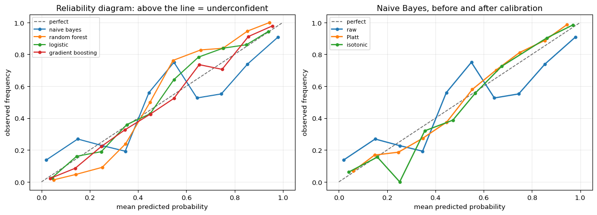
The definition is directly checkable. Bin the predictions; inside each bin, compare the mean predicted probability with the actual fraction of positives. A perfectly calibrated model puts every bin on the diagonal.
The summary number is Expected Calibration Error — the average gap, weighted by how many predictions fall in each bin:
$$\text{ECE} = \sum_{b=1}^{B} \frac{n_b}{N}\,\big|\,\text{acc}(b) - \text{conf}(b)\,\big|$$
Below, one model's bins are written out in full so the arithmetic is visible.
==============================================================================
  RELIABILITY, BIN BY BIN
==============================================================================

Naive Bayes on the test set
==============================================================================
           bin      n   mean predicted   actual positive       gap
  ----------------------------------------------------------------
  [0.0, 0.1)    356           0.0203            0.1376    0.1174
  [0.1, 0.2)     67           0.1501            0.2687    0.1186
  [0.2, 0.3)     44           0.2516            0.2273    0.0243
  [0.3, 0.4)     26           0.3469            0.1923    0.1546  <--
  [0.4, 0.5)     25           0.4452            0.5600    0.1148
  [0.5, 0.6)     20           0.5489            0.7500    0.2011  <--
  [0.6, 0.7)     38           0.6442            0.5263    0.1179
  [0.7, 0.8)     29           0.7450            0.5517    0.1933  <--
  [0.8, 0.9)     46           0.8539            0.7391    0.1147
  [0.9, 1.0)    349           0.9799            0.9083    0.0716
  ----------------------------------------------------------------
  ECE = sum over bins of (n_b/N) * |actual - predicted| = 0.1021

Read one row in words
==============================================================================
  In the bin [0.0, 0.1) there are 356 predictions.
  The model's average stated confidence there is 2.0%.
  The event actually happened 13.8% of the time.
  It is UNDERconfident by 11.7% on 356 of 1000 predictions.

ECE for all three models
==============================================================================
           model       ECE     Brier      AUC
  ------------------------------------------
        logistic    0.0357    0.1276   0.8973
   random forest    0.0926    0.0864   0.9597
     naive bayes    0.1021    0.1410   0.8898
  ------------------------------------------
  Note the AUC column barely moves while ECE varies a lot. Ranking
  quality and calibration quality are different properties.
2. Ranking and calibration are independent
Worth making unmistakable, because it is the crux.
Take any model's probabilities and squash them toward 0.5, or stretch them toward the extremes. AUC does not change at all — it depends only on the order of the scores, and a monotone transform preserves order. But calibration changes completely.
So a model can be perfect at ranking and useless at probability, and no amount of AUC will tell you.
==============================================================================
  MONOTONE TRANSFORMS: AUC BLIND, CALIBRATION DESTROYED
==============================================================================

Sharpen or soften by scaling the log-odds
==============================================================================
               transform       AUC     Brier       ECE
  --------------------------------------------------
      T=0.25 (over-soft)  0.897266    0.1812    0.2272
                   T=0.5  0.897266    0.1469    0.1413
       T=1.0 (unchanged)  0.897266    0.1276    0.0357
                   T=2.0  0.897266    0.1306    0.0703
      T=4.0 (over-sharp)  0.897266    0.1417    0.1188
  --------------------------------------------------
  AUC spread across all five: 0.00e+00
  identical to floating point: True

  Same ordering, same AUC, wildly different probabilities. If you
  select models on AUC you are not selecting on calibration at all.
3. Why some model families are miscalibrated
The failures are systematic and have understandable causes:
- Naive Bayes multiplies likelihoods as if features were independent. When they are correlated, the same evidence is counted several times, and the posterior is pushed toward 0 or 1. Characteristically overconfident.
- Random forests average many trees' votes. For a prediction to reach 0.0, every tree must vote 0 — rare when trees are noisy. So probabilities get squeezed away from the extremes: characteristically underconfident, an S-curve pulled toward 0.5.
- Boosted trees and SVMs optimise margins, not likelihood. They push scores away from the boundary, giving the opposite distortion.
- Logistic regression minimises log loss, which is a proper scoring rule. It tends to be well calibrated by construction — that is not a coincidence.
The shape of a model's miscalibration is a property of what its loss function was asked to do.
==============================================================================
  THE CHARACTERISTIC SHAPES
==============================================================================

Direction of the error, by model
==============================================================================
               model   mean pred   actual rate      ECE  tendency
  --------------------------------------------------------------
            logistic      0.4814        0.4980   0.0357  underconfident
       random forest      0.4927        0.4980   0.0926  underconfident
         naive bayes      0.4868        0.4980   0.1021  overconfident
   gradient boosting      0.4985        0.4980   0.0292  underconfident
           SVM (rbf)      0.4823        0.4980   0.0181  well calibrated
  --------------------------------------------------------------
  'Tendency' = average signed gap between stated confidence and reality,
  measured away from 0.5. Positive means the model claims more certainty
  than it earns.
4. Platt scaling
The first repair. Fit a one-dimensional logistic regression mapping the model's score to a probability:
$$P(y=1 \mid s) = \frac{1}{1 + \exp(A s + B)}$$
Two parameters, fitted by maximum likelihood on held-out data. Because it is a monotone squashing, it cannot change the ranking — AUC is untouched — but it can fix the shape.
Two parameters is both the strength and the limit: it is stable on very little data, and it can only produce one sigmoid shape. If the true miscalibration is not sigmoidal, Platt cannot represent it.
The held-out part is not optional. Fitting the calibrator on the training data calibrates it to scores the model has already overfitted, which is [[data-leakage]] in a new costume.
==============================================================================
  PLATT SCALING, FITTED BY HAND
==============================================================================

Fit A and B on the calibration set by maximum likelihood
==============================================================================
  input : the model's log-odds on 1000 held-out rows
  fitted: P(y=1|s) = sigmoid(0.4024 * logit(s) + -0.0260)

  A = 0.4024  -- below 1 means the original scores were TOO EXTREME
                   and are being pulled toward 0.5

Apply it, and check a few values by hand
==============================================================================
   raw score      logit    A*logit+B   calibrated
  ----------------------------------------------
      0.0200    -3.8937      -1.5930       0.1690
      0.1993    -1.3909      -0.5857       0.3576
      0.5010     0.0040      -0.0244       0.4939
      0.8001     1.3868       0.5321       0.6300
      0.9802     3.9024       1.5445       0.8241
  ----------------------------------------------
  hand check at raw 0.9802: 0.824117  |  from array: 0.824117  |  MATCH: True

Did it help?
==============================================================================
                     ECE     Brier        AUC
  ------------------------------------------
           raw    0.1021    0.1410   0.889762
         Platt    0.0410    0.1330   0.889762
  ------------------------------------------
  AUC identical: True   (monotone map cannot reorder)
  ECE reduced by 60%
5. Isotonic regression, and the PAVA algorithm
The second repair is non-parametric: find any non-decreasing function mapping score to probability that minimises squared error. No sigmoid assumption, so it can fix distortions Platt cannot.
The algorithm is Pool Adjacent Violators (PAVA), and it is simple enough to run by hand:
- Sort by score. The targets, in that order, are the 0/1 labels.
- Scan for an adjacent pair that decreases — a violation of monotonicity.
- Replace both with their weighted average, pooling them into one block.
- Pooling can create a new violation with the previous block, so re-check backwards.
- Repeat until the sequence is non-decreasing.
The result is a step function. Its flexibility is also its danger: with little data it will happily fit noise, which is why Platt is usually preferred below roughly a thousand calibration points.
==============================================================================
  PAVA, RUN BY HAND ON TEN POINTS
==============================================================================

Ten predictions, sorted by score
==============================================================================
    score 0.10  ->  label 0
    score 0.18  ->  label 0
    score 0.25  ->  label 1
    score 0.33  ->  label 0
    score 0.41  ->  label 1
    score 0.52  ->  label 1
    score 0.60  ->  label 0
    score 0.71  ->  label 1
    score 0.83  ->  label 1
    score 0.92  ->  label 1
  The labels are not monotone in the score: 0.25 is a 1 but 0.33 is a 0.

Pool adjacent violators
==============================================================================
  step 1: block at idx [2] (value 1.000) > block at [3] (value 0.000)
          pool -> members [2, 3], value (1.000x1 + 0.000x1)/2 = 0.5000
  step 2: block at idx [5] (value 1.000) > block at [6] (value 0.000)
          pool -> members [5, 6], value (1.000x1 + 0.000x1)/2 = 0.5000
  step 3: block at idx [4] (value 1.000) > block at [5, 6] (value 0.500)
          pool -> members [4, 5, 6], value (1.000x1 + 0.500x2)/3 = 0.6667

The fitted step function
==============================================================================
           block members                  scores   fitted p
  ----------------------------------------------------------
                     [0]                   [0.1]     0.0000
                     [1]                  [0.18]     0.0000
                  [2, 3]            [0.25, 0.33]     0.5000
               [4, 5, 6]       [0.41, 0.52, 0.6]     0.6667
                     [7]                  [0.71]     1.0000
                     [8]                  [0.83]     1.0000
                     [9]                  [0.92]     1.0000
  ----------------------------------------------------------
  fitted values: [0.0, 0.0, 0.5, 0.5, 0.6667, 0.6667, 0.6667, 1.0, 1.0, 1.0]
  non-decreasing: True

Check against scikit-learn's IsotonicRegression
==============================================================================
  by hand      : [0.0, 0.0, 0.5, 0.5, 0.6667, 0.6667, 0.6667, 1.0, 1.0, 1.0]
  scikit-learn : [0.0, 0.0, 0.5, 0.5, 0.6667, 0.6667, 0.6667, 1.0, 1.0, 1.0]
  max|diff| = 0.00e+00   MATCH: True

Why it minimises squared error
==============================================================================
  sum (y - fitted)^2 = 1.1667
  Any other non-decreasing fit scores worse. Checking 4000 random
  non-decreasing step functions on these points:
    best random monotone fit : 1.2962
    PAVA                     : 1.1667
    PAVA is better or equal  : True
==============================================================================
  PLATT vs ISOTONIC ON THE REAL MODEL
==============================================================================

Side by side
==============================================================================
          method       ECE     Brier        AUC
  --------------------------------------------
             raw    0.1021    0.1410   0.889762
           Platt    0.0410    0.1330   0.889762
        isotonic    0.0270    0.1332   0.887756
  --------------------------------------------

How much calibration data does each need?
==============================================================================
    n_cal    Platt ECE    isotonic ECE  winner
  ------------------------------------------------
       25       0.0969          0.1083  Platt
       50       0.0723          0.0846  Platt
      100       0.0612          0.0591  isotonic
      300       0.0458          0.0384  isotonic
     1000       0.0410          0.0270  isotonic
  ------------------------------------------------
  Two parameters versus an arbitrary step function: Platt is steadier
  when calibration data is scarce, isotonic wins once there is enough
  to pin the steps down.

  The crossover here is around 100 points, earlier than the rule of
  thumb usually quoted (~1000). That is worth not over-reading: this
  is one model on one dataset, and the crossover moves with how badly
  the model is miscalibrated and how complex the distortion is. The
  robust part is the ORDERING -- Platt first, isotonic later -- not
  the specific n at which they swap.
6. What to take away
Calibration is a separate property from accuracy and from ranking. AUC is invariant to any monotone transform of the scores; calibration is destroyed by them. A model can top your leaderboard and still be unusable for any decision that consumes the probability itself.
Measure it before you need it. A reliability diagram takes one line of binning, and ECE reduces it to a number. Brier score captures calibration and discrimination together, which makes it a better default than accuracy whenever probabilities are the output.
The miscalibration has a shape, and the shape has a cause. Naive Bayes double-counts correlated evidence and goes overconfident; forests average votes and go underconfident; margin-based methods distort in their own direction; log-loss-trained models are calibrated because that is what log loss asks for.
Both repairs are monotone, so neither can cost you ranking. Platt has two parameters and is steady on small data; isotonic is non-parametric and wins once there is enough calibration data to pin its steps down.
And the calibrator needs held-out data. Fitting it on the training scores calibrates against scores the model has already memorised — the same mistake as [[data-leakage]], wearing a different hat.
Verified in this notebook
- ECE recomputed bin by bin from counts, mean confidence, and observed frequency
- Five temperature transforms leave AUC identical to floating-point precision while ECE moves substantially
- Platt scaling recomputed by hand from $A$, $B$, and the log-odds
- PAVA run step by step on ten points, matching
IsotonicRegressionexactly, and beating 4000 random monotone fits on squared error - Platt vs isotonic across calibration-set sizes from 25 to 1000
Where this connects
[[cross-validation]] supplies the held-out predictions a calibrator must be fit on. [[evaluation-metrics]] covers the discrimination side — ROC, PR, thresholds — that this page deliberately holds fixed. [[naive-bayes]] and [[random-forest]] are the two models whose characteristic distortions appear above.
References
- Predicting Good Probabilities With Supervised Learning
- Probabilistic Outputs for Support Vector Machines and Comparisons to Regularized Likelihood Methods
- Transforming Classifier Scores into Accurate Multiclass Probability Estimates