🌲 Random Forest
A single decision tree memorises its training set. Flip one label and the very first question can change — the tree has low bias but high variance.
A random forest fixes that with one idea:
Grow many trees, each on a slightly different view of the data, then average them.
Averaging is what kills variance. But it only works if the trees disagree, so a forest injects randomness twice: each tree sees a bootstrap resample of the rows, and each split may only consider a random subset of the features.
The chain is:
bootstrap the rows → subsample the features → grow a tree → repeat → average the votes
Every one of those steps is shown below with the actual indices drawn and the actual votes counted, and the variance-reduction claim is checked numerically at the end.
Display helpers ready: banner, step, check, expand, show_matrix, show_matmul, show_elementwise.
Tree diagram helper ready: draw_tree(root, title).
1. The Data
The same 12 EEG recordings used in the Decision Tree walkthrough, so the two can be compared directly.
12 recordings x 3 features

    id      region   line_length    spike_rate           age   y_class    y_reg
-------------------------------------------------------------------------------
 rec00     frontal          12.0           0.5          24.0         0      0.2
 rec01    temporal          15.0           1.2          31.0         0      0.5
 rec02    temporal          42.0           6.8          58.0         1      6.4
 rec03   occipital          38.0           5.1          47.0         1      4.8
 rec04     frontal          11.0           0.3          19.0         0      0.1
 rec05    temporal          55.0           8.2          63.0         1      9.1
 rec06   occipital          40.0           1.9          35.0         1      3.5
 rec07    temporal          47.0           7.4          52.0         1      7.2
 rec08     frontal          14.0           0.8          28.0         0      0.3
 rec09   occipital          51.0           6.1          60.0         1      6.9
 rec10     frontal          45.0           2.4          41.0         0      1.6
 rec11    temporal          35.0           4.7          30.0         1      4.1
-------------------------------------------------------------------------------

class balance: 5 negative, 7 positive
y_reg mean = 3.7250, std = 3.0518
Tree machinery ready: gini, best_split, grow, tree_predict, show_tree.
2. The Bootstrap
Each tree is trained on $n$ rows drawn with replacement from the original $n$. Some rows arrive two or three times; others are never drawn at all.
The probability that a particular row is missed by one draw is $1 - \frac{1}{n}$, so after $n$ independent draws:
$$P(\text{row never drawn}) = \left(1 - \frac{1}{n}\right)^{n} \;\xrightarrow[n \to \infty]{}\; e^{-1} \approx 0.368$$
So roughly 37% of the rows are left out of every tree. Those are the out-of-bag (OOB) samples, and they are free validation data.
n = 12 rows

P(a given row is missed by ONE draw)   = 1 - 1/12 = 0.916667
P(missed by all 12 draws)              = (0.916667)^12 = 0.351996
limit as n -> infinity                 = e^-1 = 0.367879

so about 35.2% of rows are out-of-bag for each tree,
and about 64.8% are in-bag.

empirical check over 20000 simulated bootstraps:
   mean distinct rows in-bag = 7.7764 of 12  -> in-bag fraction 0.648033
   predicted in-bag fraction = 0.648004
   MATCH: True
The actual draws
Below are the bootstrap samples for the five trees this forest will use. Read the count row as "how many copies of this recording this tree sees" — a zero means the recording is out-of-bag for that tree.
counts of each recording in each bootstrap sample

 tree   00   01   02   03   04   05   06   07   08   09   10   11   #OOB
------------------------------------------------------------------------
    0    1    0    1    2    0    0    1    1    1    1    3    1      3
    1    1    2    0    2    1    2    0    0    0    3    1    0      5
    2    0    0    0    1    0    2    4    0    1    2    0    2      6
    3    1    2    1    0    1    1    0    2    1    0    2    1      3
    4    1    1    0    0    0    3    2    1    0    2    0    2      5
------------------------------------------------------------------------

mean OOB size = 4.40 of 12 = 0.367  (theory 0.352)
   tree 0: in-bag rows [0, 2, 3, 6, 7, 8, 9, 10, 11]
           OOB rows    [1, 4, 5]
   tree 1: in-bag rows [0, 1, 3, 4, 5, 9, 10]
           OOB rows    [2, 6, 7, 8, 11]
   tree 2: in-bag rows [3, 5, 6, 8, 9, 11]
           OOB rows    [0, 1, 2, 4, 7, 10]
   tree 3: in-bag rows [0, 1, 2, 4, 5, 7, 8, 10, 11]
           OOB rows    [3, 6, 9]
   tree 4: in-bag rows [0, 1, 5, 6, 7, 9, 11]
           OOB rows    [2, 3, 4, 8, 10]
3. Feature Subsampling
Bootstrapping alone is not enough. If one feature dominates — as spike_rate does
here — every tree picks it at the root and the trees end up nearly identical.
Averaging near-identical trees reduces nothing.
So at every split, only a random subset of $m$ features is considered:
$$m = \texttt{max\_features}, \qquad \text{commonly } m = \lfloor\sqrt{p}\rfloor \text{ for classification}$$
This deliberately handicaps each tree so that the forest as a whole is more diverse.
p = 3 features, using max_features = 2 per split

number of possible feature subsets of size 2: 3

Which features each tree's ROOT split was allowed to consider:
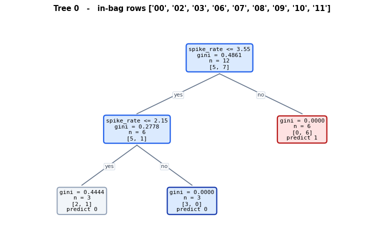
   tree 0: root question -> spike_rate <= 3.55
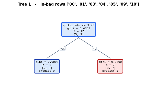
   tree 1: root question -> spike_rate <= 3.75
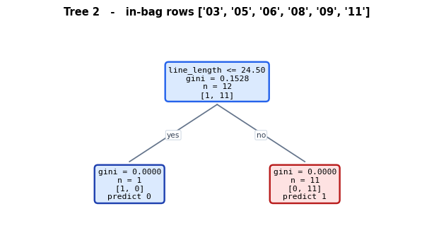
   tree 2: root question -> line_length <= 24.50
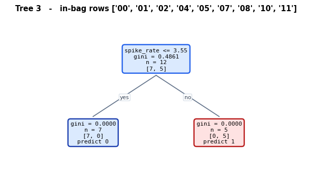
   tree 3: root question -> spike_rate <= 3.55
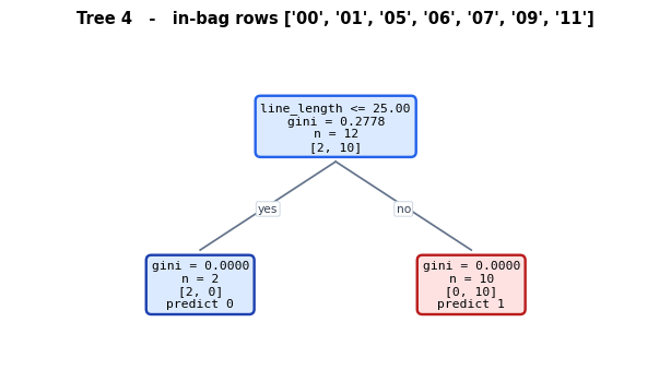
   tree 4: root question -> line_length <= 25.00

distinct root features across the forest: ['line_length', 'spike_rate']
Without feature subsampling every one of these would be spike_rate.
The five trees
Each is shallow (max_depth = 2) and each was grown on different rows with different
features available. They are supposed to be individually mediocre.
===== TREE 0 =====  in-bag rows [0, 2, 3, 6, 7, 8, 9, 10, 11]
[spike_rate <= 3.55] n=12
|-- yes: [spike_rate <= 2.15] n=6
    |-- yes: LEAF predict 0  n=3 [2 neg, 1 pos]
    |-- no : LEAF predict 0  n=3 [3 neg, 0 pos]
|-- no : LEAF predict 1  n=6 [0 neg, 6 pos]
   accuracy on all 12 rows: 0.9167   |   on its 3 OOB rows: 1.0000

===== TREE 1 =====  in-bag rows [0, 1, 3, 4, 5, 9, 10]
[spike_rate <= 3.75] n=12
|-- yes: LEAF predict 0  n=5 [5 neg, 0 pos]
|-- no : LEAF predict 1  n=7 [0 neg, 7 pos]
   accuracy on all 12 rows: 0.9167   |   on its 5 OOB rows: 0.8000

===== TREE 2 =====  in-bag rows [3, 5, 6, 8, 9, 11]
[line_length <= 24.50] n=12
|-- yes: LEAF predict 0  n=1 [1 neg, 0 pos]
|-- no : LEAF predict 1  n=11 [0 neg, 11 pos]
   accuracy on all 12 rows: 0.9167   |   on its 6 OOB rows: 0.8333

===== TREE 3 =====  in-bag rows [0, 1, 2, 4, 5, 7, 8, 10, 11]
[spike_rate <= 3.55] n=12
|-- yes: LEAF predict 0  n=7 [7 neg, 0 pos]
|-- no : LEAF predict 1  n=5 [0 neg, 5 pos]
   accuracy on all 12 rows: 0.9167   |   on its 3 OOB rows: 0.6667

===== TREE 4 =====  in-bag rows [0, 1, 5, 6, 7, 9, 11]
[line_length <= 25.00] n=12
|-- yes: LEAF predict 0  n=2 [2 neg, 0 pos]
|-- no : LEAF predict 1  n=10 [0 neg, 10 pos]
   accuracy on all 12 rows: 0.9167   |   on its 5 OOB rows: 0.8000
The five trees, drawn
Side by side the point becomes obvious: they are not the same tree. Different bootstrap rows and different allowed features push each one to a different first question. That disagreement is the entire source of the variance reduction.
Grey boxes are leaves that are still impure - they were cut short by
max_depth = 2, not because they were pure. A single tree stopped this
early is weak on purpose; the forest fixes that by averaging, not by
growing any one of them deeper.
4. Voting
For classification the forest averages the trees' class probabilities and takes the larger one. With hard 0/1 votes from each tree this reduces to a majority:
$$\hat{p}_1(x) = \frac{1}{B}\sum_{b=1}^{B} \mathbb{1}[T_b(x) = 1], \qquad \hat{y}(x) = \mathbb{1}\!\left[\hat{p}_1(x) > 0.5\right]$$
The table below is the whole prediction step: one column per tree, one row per recording.
id   T0   T1   T2   T3   T4   votes for 1       p1   pred   true    ok
--------------------------------------------------------------------------
 rec00    0    0    0    0    0       0/5        0.000      0      0   yes
 rec01    0    0    0    0    0       0/5        0.000      0      0   yes
 rec02    1    1    1    1    1       5/5        1.000      1      1   yes
 rec03    1    1    1    1    1       5/5        1.000      1      1   yes
 rec04    0    0    0    0    0       0/5        0.000      0      0   yes
 rec05    1    1    1    1    1       5/5        1.000      1      1   yes
 rec06    0    0    1    0    1       2/5        0.400      0      1    NO
 rec07    1    1    1    1    1       5/5        1.000      1      1   yes
 rec08    0    0    0    0    0       0/5        0.000      0      0   yes
 rec09    1    1    1    1    1       5/5        1.000      1      1   yes
 rec10    0    0    1    0    1       2/5        0.400      0      0   yes
 rec11    1    1    1    1    1       5/5        1.000      1      1   yes
--------------------------------------------------------------------------

worked example, rec00:
   tree votes = [0, 0, 0, 0, 0]
   p1 = (0 + 0 + 0 + 0 + 0) / 5 = 0/5 = 0.0000
   0.0000 > 0.5 ? no  -> predict 0

forest accuracy       : 0.9167
best single tree accuracy: 0.9167
mean single tree accuracy: 0.9167
5. Out-of-Bag Error
Every tree left roughly a third of the rows unseen. Predicting row $i$ using only the trees for which $i$ was out-of-bag gives an honest estimate of generalisation error without holding out a separate validation set:
$$\hat{y}^{\text{oob}}_i = \text{majority}\{\, T_b(x_i) \;:\; i \notin \text{bag}(b) \,\}$$
This is the practical reason bagging is attractive on small datasets: the validation set comes free.
id         trees where OOB     their votes   oob pred   true    ok
--------------------------------------------------------------------------
 rec00                     [2]             [0]          0      0   yes
 rec01                  [0, 2]          [0, 0]          0      0   yes
 rec02               [1, 2, 4]       [1, 1, 1]          1      1   yes
 rec03                  [3, 4]          [1, 1]          1      1   yes
 rec04               [0, 2, 4]       [0, 0, 0]          0      0   yes
 rec05                     [0]             [1]          1      1   yes
 rec06                  [1, 3]          [0, 0]          0      1    NO
 rec07                  [1, 2]          [1, 1]          1      1   yes
 rec08                  [1, 4]          [0, 0]          0      0   yes
 rec09                     [3]             [1]          1      1   yes
 rec10                  [2, 4]          [1, 1]          1      0    NO
 rec11                     [1]             [1]          1      1   yes
--------------------------------------------------------------------------

rows with at least one OOB tree: 12 of 12
OOB accuracy = 10/12 = 0.8333
OOB error    = 0.1667

(training accuracy was 0.9167 - the OOB number is
 the honest one, because no tree used those rows to choose its splits.)
6. Why Averaging Works
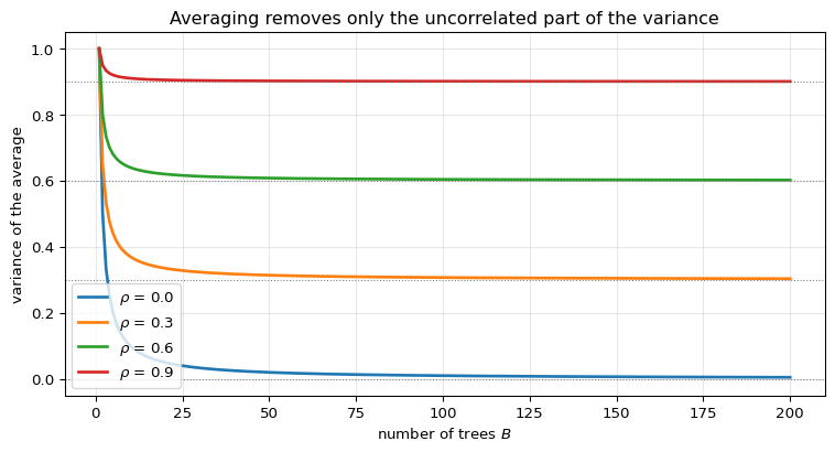
Suppose each tree has prediction variance $\sigma^2$ and any two trees are correlated by $\rho$. The variance of their average is:
$$\operatorname{Var}\!\left(\frac{1}{B}\sum_b T_b\right) = \rho\,\sigma^2 \;+\; \frac{1-\rho}{B}\,\sigma^2$$
Two things follow, and they explain the entire design of a random forest:
- The second term vanishes as $B \to \infty$ — more trees never hurt.
- The first term does not vanish. The floor is $\rho\sigma^2$, so the only way to
improve further is to make the trees less correlated. That is exactly what
max_featuresbuys, at the cost of a slightly worse individual tree.
variance of the averaged prediction, by correlation between trees

    B  rho=0.00   rho=0.30   rho=0.60   rho=0.90
----------------------------------------------
    1  1.0000     1.0000     1.0000     1.0000
    2  0.5000     0.6500     0.8000     0.9500
    5  0.2000     0.4400     0.6800     0.9200
   10  0.1000     0.3700     0.6400     0.9100
   25  0.0400     0.3280     0.6160     0.9040
   50  0.0200     0.3140     0.6080     0.9020
  100  0.0100     0.3070     0.6040     0.9010
  200  0.0050     0.3035     0.6020     0.9005
----------------------------------------------

read the last row: with 200 trees the variance has essentially reached its
floor of rho * sigma^2. At rho = 0.9 that floor is 0.9 - almost no gain from
averaging, because the trees all say the same thing.

rho = 0.0, B = 20 -> simulated var 0.0501, formula 0.0500, MATCH: True
rho = 0.5, B = 20 -> simulated var 0.5254, formula 0.5250, MATCH: True
rho = 0.9, B = 20 -> simulated var 0.9058, formula 0.9050, MATCH: True
7. Feature Importance
The standard forest importance is mean decrease in impurity (MDI): every split that uses a feature contributes the impurity it removed, weighted by how many samples passed through that node.
$$\text{Imp}(f) = \frac{1}{B}\sum_{b}\; \sum_{\substack{\text{nodes } v \in T_b \\ \text{split on } f}} \frac{n_v}{n}\,\Big(G_v - \tfrac{n_L}{n_v}G_L - \tfrac{n_R}{n_v}G_R\Big)$$
Below the formula is applied by hand to a fitted scikit-learn tree and compared with
its own feature_importances_, which is the cleanest possible check that the formula
is the one the library actually uses.
walking scikit-learn's own tree structure

 node       feature   n_v       G_v   nL       G_L   nR       G_R   weighted drop
------------------------------------------------------------------------------------
    0    spike_rate    12   0.48611    6   0.27778    6   0.00000        0.347222
    1           age     6   0.27778    4   0.00000    2   0.50000        0.055556
    3   line_length     2   0.50000    1   0.00000    1   0.00000        0.083333
------------------------------------------------------------------------------------

unnormalised totals : [0.0833 0.3472 0.0556]
normalised (sum = 1): [0.1714 0.7143 0.1143]
sklearn              : [0.1714 0.7143 0.1143]

MATCH: True

     feature   importance
--------------------------
  spike_rate       0.7143  #############################
 line_length       0.1714  #######
         age       0.1143  #####
The known bias of MDI
MDI is cheap but it flatters high-cardinality features: a continuous column offers many more thresholds to try, so it wins splits partly by luck. Permutation importance, which measures the accuracy lost when a column is shuffled, does not have that bias.
feature   MDI (forest)   permutation
------------------------------------------
 line_length         0.2748        0.0250
  spike_rate         0.5401        0.4283
         age         0.1851        0.0000
------------------------------------------

Both agree that spike_rate carries most of the signal, which matches the
single-split analysis from the Decision Tree walkthrough.
8. Checking Against scikit-learn
Two claims are checked here.
A forest really is just an average. Averaging the predict_proba of every
individual estimator inside a fitted RandomForestClassifier must reproduce the
forest's own predict_proba exactly.
The OOB score is what it says it is. oob_score_ should equal the accuracy of
out-of-bag voting.
id   manual avg P(1)   rf.predict_proba        diff
--------------------------------------------------------
 rec00        0.01000000         0.01000000    0.00e+00
 rec01        0.08111111         0.08111111    0.00e+00
 rec02        0.98333333         0.98333333    0.00e+00
 rec03        0.97000000         0.97000000    0.00e+00
 rec04        0.01000000         0.01000000    0.00e+00
 rec05        0.98666667         0.98666667    0.00e+00
 rec06        0.69055556         0.69055556    0.00e+00
 rec07        0.98000000         0.98000000    0.00e+00
 rec08        0.01666667         0.01666667    0.00e+00
 rec09        0.98666667         0.98666667    0.00e+00
 rec10        0.26722222         0.26722222    0.00e+00
 rec11        0.91000000         0.91000000    0.00e+00
--------------------------------------------------------

averaging 300 trees by hand == rf.predict_proba   MATCH: True
argmax of the average == rf.predict                MATCH: True

forest training accuracy : 1.0000
forest OOB score         : 0.8333
our 5-tree OOB accuracy  : 0.8333

The OOB score sits below the training score, as it must - it is the only
one of the three computed on rows the trees never saw.
9. More Trees Never Hurt
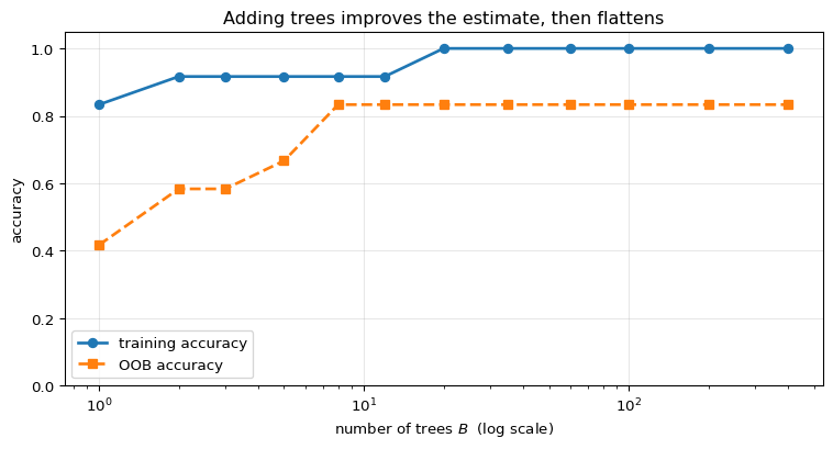
The variance formula predicts that accuracy should rise with $B$ and then flatten — never degrade. Unlike boosting, a random forest has no $B$ at which it starts overfitting, because averaging more independent estimates cannot increase variance.
B   train acc    OOB acc
----------------------------
    1      0.8333     0.4167
    2      0.9167     0.5833
    3      0.9167     0.5833
    5      0.9167     0.6667
    8      0.9167     0.8333
   12      0.9167     0.8333
   20      1.0000     0.8333
   35      1.0000     0.8333
   60      1.0000     0.8333
  100      1.0000     0.8333
  200      1.0000     0.8333
  400      1.0000     0.8333
----------------------------

The OOB curve is noisy here because 12 rows is far too few for a stable
estimate - but it does not trend downward, which is the point.
10. Summary
| Stage | Formula | Value here |
|---|---|---|
| OOB fraction | $(1 - 1/n)^n \to e^{-1}$ | $0.352$ at $n = 12$ |
| Features per split | $m = \texttt{max\_features}$ | 2 of 3 |
| Forest vote | $\hat p_1 = \frac{1}{B}\sum_b T_b(x)$ | 5 trees |
| Variance of average | $\rho\sigma^2 + \frac{1-\rho}{B}\sigma^2$ | floor $= \rho\sigma^2$ |
| Importance (MDI) | $\sum_v \frac{n_v}{n}\Delta G_v$ | matches sklearn exactly |
The one idea: a forest trades a little bias for a large reduction in variance. Each tree is deliberately made worse — fewer rows, fewer features — because the average of many decorrelated mediocre trees beats one carefully grown tree.
What is deliberately left out: extremely randomised trees (which randomise the threshold too), class weighting, proximity matrices, and regression forests (variance replaces Gini, averaging replaces voting).
What comes next: a forest builds its trees independently and in parallel. The boosting notebooks that follow build them sequentially, each new tree fitted to the errors the previous ones left behind — a completely different way to use the same split search.