🔄 RNN & LSTM
A dense network sees a fixed-size input and has no notion of "before". A convolution sees a fixed window. Neither can answer "has this pattern been building up for the last two seconds?" — and for EEG, speech, or text, that is usually the question.
A recurrent network adds one thing: a hidden state carried from one timestep to the next.
$$\mathbf{h}_t = \tanh\big(W_x\mathbf{x}_t + W_h\mathbf{h}_{t-1} + \mathbf{b}\big)$$
That is the entire architecture. $\mathbf{h}_t$ is a summary of everything seen so far, $\mathbf{h}_{t-1}$ carries it forward, and the same weights are used at every timestep — parameter sharing across time rather than across space.
It also has a specific, famous failure. Because the same $W_h$ is applied at every step, gradients flowing back through $T$ steps are multiplied by $W_h$ roughly $T$ times, so they vanish or explode geometrically. That failure is measured below, and it is exactly what the LSTM was invented to fix.
Display helpers ready: banner, step, check, expand, show_matrix, show_matmul, show_elementwise.
Network diagram helper ready: draw_network(layer_sizes, Ws, bs, ...).
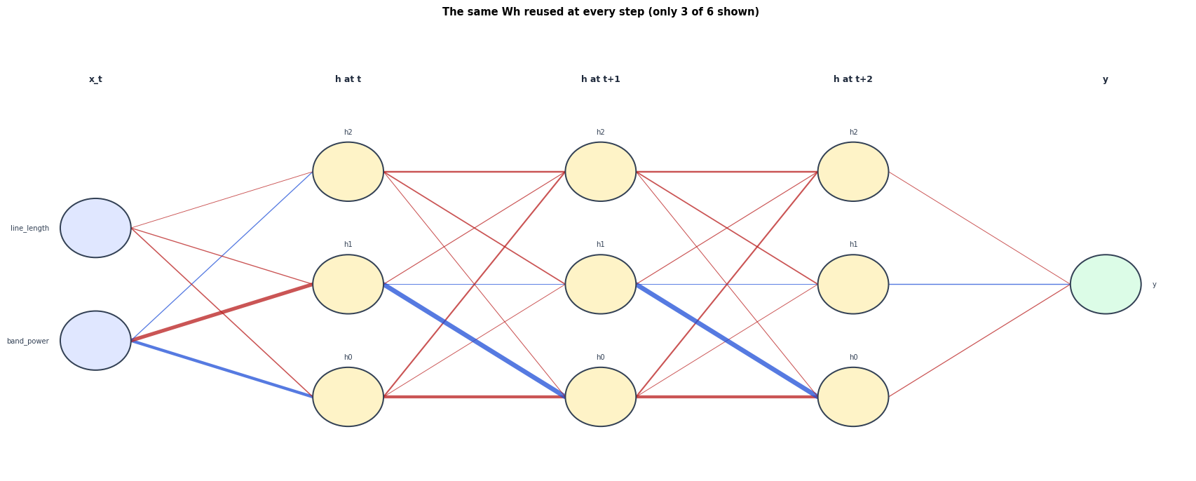
   edge width = |weight|,  blue = positive,  red = negative
1. The Sequence
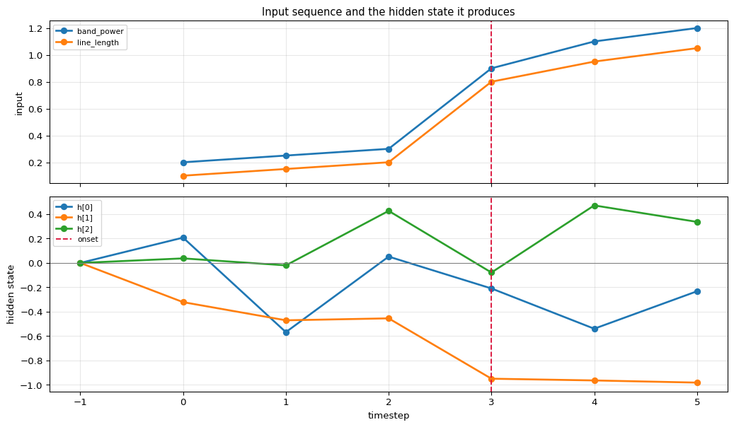
A short EEG-like sequence: 6 timesteps, 2 features per step (say band power and line length). The task is to say whether a seizure is underway by the end — a decision that depends on the history, not on the final timestep alone.
one sequence: 6 timesteps x 2 features

  step     band_power    line_length
----------------------------------------
    t0           0.20           0.10
    t1           0.25           0.15
    t2           0.30           0.20
    t3           0.90           0.80   <- onset
    t4           1.10           0.95
    t5           1.20           1.05
----------------------------------------

target: 1 (seizure)   - a property of the WHOLE sequence

Note what a plain feed-forward net would have to do: either look at one
timestep (losing the history) or flatten all 6 into a 12-long vector,
which fixes the length forever and learns each position separately.
2. The RNN Cell, Unrolled
The cell is applied once per timestep, always with the same weights:
$$\mathbf{h}_t = \tanh\big(W_x\mathbf{x}_t + W_h\mathbf{h}_{t-1} + \mathbf{b}\big), \qquad \mathbf{h}_{-1} = \mathbf{0}$$
Drawing it "unrolled" makes the structure obvious: it is a deep network whose depth equals the sequence length, and whose layers are forced to share one weight matrix.
weights - and there is only ONE set, reused at every timestep

Wx  (input -> hidden) (2, 3) =
                     h0        h1        h2
   band_power |   +1.225    -1.533    +0.251
   line_length |   -0.341    -0.272    -0.129

Wh  (hidden -> hidden) (3, 3) =
                     h0        h1        h2
           h0 |   -1.212    -0.139    -0.519
           h1 |   +1.994    +0.135    -0.212
           h2 |   -0.169    -0.401    -0.633

parameters: Wx 6 + Wh 9 + bh 3 + Wy 3 + by 1 = 22
and that count does NOT change if the sequence becomes 1000 steps long.


unrolling, one timestep at a time
==============================================================================

--- t = 0 ---   x_t = [0.2 0.1]
   x_t @ Wx        = [ 0.2108 -0.3338  0.0372]
   h_prev @ Wh     = [0. 0. 0.]      (h_prev = [0. 0. 0.])
   z = sum + bias  = [ 0.2108 -0.3338  0.0372]
   h_t = tanh(z)   = [ 0.2078 -0.322   0.0372]

   worked element h_0[0]:
      (+0.2000)*(+1.2246) + (+0.1000)*(-0.3407)
      = +0.210844   (h_prev is all zeros, adds nothing)
      tanh(+0.210844) = +0.207774   MATCH: True

--- t = 1 ---   x_t = [0.25 0.15]
   x_t @ Wx        = [ 0.255  -0.4241  0.0433]
   h_prev @ Wh     = [-0.9    -0.0874 -0.0633]      (h_prev = [ 0.2078 -0.322   0.0372])
   z = sum + bias  = [-0.645  -0.5115 -0.02  ]
   h_t = tanh(z)   = [-0.5683 -0.4711 -0.02  ]

--- t = 2 ---   x_t = [0.3 0.2]
   x_t @ Wx        = [ 0.2992 -0.5143  0.0494]
   h_prev @ Wh     = [-0.2472  0.0233  0.4074]      (h_prev = [-0.5683 -0.4711 -0.02  ])
   z = sum + bias  = [ 0.052  -0.4911  0.4567]
   h_t = tanh(z)   = [ 0.052  -0.4551  0.4274]

--- t = 3 ---   x_t = [0.9 0.8]
   x_t @ Wx        = [ 0.8296 -1.5973  0.1223]
   h_prev @ Wh     = [-1.0424 -0.2402 -0.2013]      (h_prev = [ 0.052  -0.4551  0.4274])
   z = sum + bias  = [-0.2129 -1.8375 -0.079 ]
   h_t = tanh(z)   = [-0.2097 -0.9506 -0.0788]

--- t = 4 ---   x_t = [1.1  0.95]
   x_t @ Wx        = [ 1.0234 -1.9447  0.1531]
   h_prev @ Wh     = [-1.6278 -0.068   0.3599]      (h_prev = [-0.2097 -0.9506 -0.0788])
   z = sum + bias  = [-0.6044 -2.0127  0.5129]
   h_t = tanh(z)   = [-0.5402 -0.9649  0.4722]

--- t = 5 ---   x_t = [1.2  1.05]
   x_t @ Wx        = [ 1.1118 -2.1252  0.1652]
   h_prev @ Wh     = [-1.3489 -0.2448  0.1856]      (h_prev = [-0.5402 -0.9649  0.4722])
   z = sum + bias  = [-0.2371 -2.3701  0.3508]
   h_t = tanh(z)   = [-0.2328 -0.9827  0.3371]

==============================================================================

final hidden state h_5 = [-0.2328 -0.9827  0.3371]
output = sigmoid(h @ Wy + by) = 0.430987   (target 1)


the hidden state over time - watch it move when the onset arrives

  step           h0           h1           h2      ||h||     change
--------------------------------------------------------------
  init     0.000000     0.000000     0.000000     0.0000
    t0     0.207774    -0.321966     0.037219     0.3850     0.3850
    t1    -0.568294    -0.471142    -0.019990     0.7385     0.7923
    t2     0.051964    -0.455064     0.427425     0.6265     0.7650
    t3    -0.209699    -0.950558    -0.078842     0.9766     0.7552
    t4    -0.540162    -0.964917     0.472238     1.2024     0.6427
    t5    -0.232767    -0.982677     0.337088     1.0646     0.3363
--------------------------------------------------------------

The biggest jump is at t3 - the step where the input changed. The state
is accumulating a summary, not just reacting to the current input.
unrolled, the RNN is a deep network with tied weights:

Every hidden-to-hidden arrow above is the SAME matrix Wh. That is what
makes it recurrent - and, as the next section shows, what makes the
gradient behave so badly.
3. Backpropagation Through Time
Training an RNN means unrolling it and running ordinary backpropagation over the unrolled graph — BPTT. One thing is different from a feed-forward net: since $W_h$ is used at every step, its gradient is the sum of the gradients from every step.
$$\frac{\partial\mathcal{L}}{\partial W_h} = \sum_{t=0}^{T-1}\frac{\partial\mathcal{L}}{\partial W_h}\bigg|_{\text{step }t}$$
And the blame at step $t$ arrives from step $t+1$ through $W_h$, scaled by the local tanh derivative:
$$\delta_t = \big(\delta_{t+1}W_h^\top\big)\odot\big(1 - \mathbf{h}_t^2\big)$$
That recursion is the source of everything that follows.
forward: y_hat = 0.430987, target = 1, loss = 0.841678

blame travelling backwards through time

  step    ||delta_t||    relative to last step
------------------------------------------------
    t5     0.14549277               100.0000%
    t4     0.14433058                99.2012%
    t3     0.18631693               128.0592%
    t2     0.36265026               249.2566%
    t1     0.38179738               262.4167%
    t0     0.35439859               243.5850%
------------------------------------------------

Each step back multiplies by Wh and by (1 - h^2). The tanh derivative is
at most 1 and usually well below it, so the blame shrinks as it travels.

   blame at the last step  : 0.14549277
   blame at the first step : 0.35439859
   ratio                   : 2.435850

Over 6 steps that is survivable. Over 100 it is not - see section 4.


gradient check against central differences (all 22 parameters)

       param         analytic        numerical      rel err
----------------------------------------------------------
    Wx[0, 0]      0.109590534      0.109590534     2.11e-11
    Wx[0, 1]      0.046428179      0.046428179     1.56e-10
    Wx[0, 2]      0.076996981      0.076996981     3.02e-10
    Wx[1, 0]      0.113044493      0.113044493     1.02e-10
    Wx[1, 1]      0.023828827      0.023828827     1.18e-10
    Wx[1, 2]      0.064431474      0.064431474     1.89e-10
         ...
----------------------------------------------------------

parameters checked : 22
worst relative error: 3.266e-09   -> CORRECT
4. Vanishing and Exploding Gradients
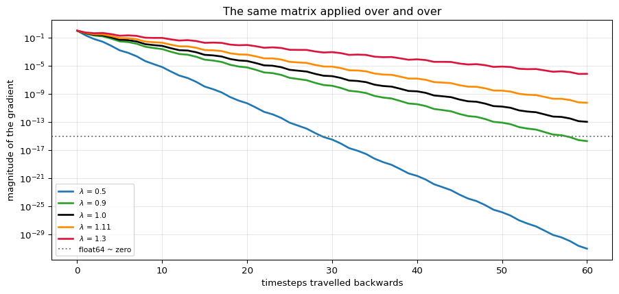
The recursion $\delta_t = (\delta_{t+1}W_h^\top)\odot(1-\mathbf{h}_t^2)$ applied $T$ times means the gradient reaching step 0 has been multiplied by roughly $W_h^T$.
$$\left\lVert\frac{\partial \mathcal{L}}{\partial \mathbf{h}_0}\right\rVert \;\sim\; \lambda^{T}, \qquad \lambda = \text{largest singular value of } W_h$$
- $\lambda < 1$ → the gradient vanishes: early timesteps receive nothing, so the network cannot learn long-range dependencies. It is not slow — it is silent.
- $\lambda > 1$ → the gradient explodes: updates become enormous and training destabilises.
The knife-edge at $\lambda = 1$ is why plain RNNs are hard to train beyond ~10–20 steps.
top singular value           T=1           T=5          T=10          T=25          T=50
------------------------------------------------------------------------------------
               0.50     2.137e-01     1.616e-03     6.725e-06     8.085e-14     1.405e-26
               0.90     3.847e-01     3.054e-02     2.401e-03     1.947e-07     8.154e-14
               1.00     4.275e-01     5.172e-02     6.886e-03     2.713e-06     1.582e-11
               1.11     4.745e-01     8.715e-02     1.955e-02     3.685e-05     2.920e-09
               1.30     5.557e-01     1.920e-01     9.494e-02     1.914e-03     7.878e-06
------------------------------------------------------------------------------------

our Wh has top singular value 2.3548
   after 6 steps  : ~1.7049e+02
   after 50 steps : ~3.9579e+18
   after 200 steps: ~2.4538e+74


what 'vanishing' means in practice, in float64:

   scale 0.5: gradient reaches 1e-15 at step 29  -> numerically ZERO beyond that
   scale 0.9: gradient reaches 1e-15 at step 58  -> numerically ZERO beyond that

   Beyond that point the early timesteps receive no learning signal at
   all. The network is not learning slowly from them; it is not learning
   from them.
Only the black line (exactly 1.0) is stable, and hitting it exactly is
not something training can be relied on to do. Everything else either
dies or blows up - geometrically.
5. The LSTM — a Gradient Highway
The LSTM's answer is not a bigger matrix. It is a second state, the cell state $\mathbf{c}_t$, whose update is additive rather than multiplicative:
$$\mathbf{c}_t = \mathbf{f}_t \odot \mathbf{c}_{t-1} \;+\; \mathbf{i}_t \odot \tilde{\mathbf{c}}_t$$
Compare the two recursions:
$$\text{RNN: } \; \mathbf{h}_t = \tanh(W_h\mathbf{h}_{t-1} + \dots) \qquad\qquad \text{LSTM: } \; \mathbf{c}_t = \mathbf{f}_t\odot\mathbf{c}_{t-1} + \dots$$
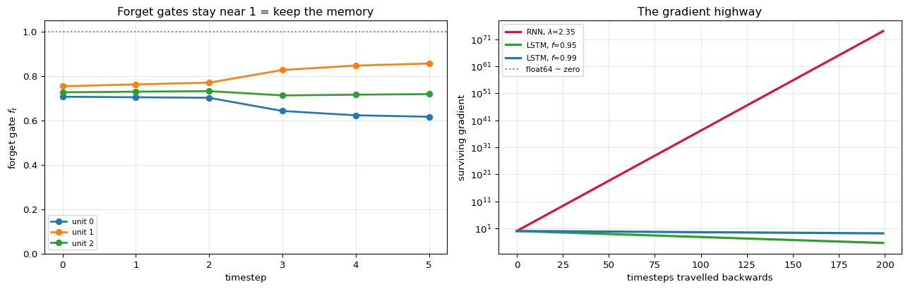
Going backwards, the RNN multiplies by $W_h$ every step. The LSTM multiplies by $\mathbf{f}_t$ — and if the forget gate is near 1, that is multiplying by one. The gradient can travel hundreds of steps essentially unchanged. That is the "constant error carousel".
Three gates control the flow, each a sigmoid producing values in $(0,1)$:
| Gate | Formula | Question it answers |
|---|---|---|
| forget $\mathbf{f}_t$ | $\sigma(W_f[\mathbf{h}_{t-1},\mathbf{x}_t] + b_f)$ | what should I discard? |
| input $\mathbf{i}_t$ | $\sigma(W_i[\dots] + b_i)$ | what new is worth storing? |
| output $\mathbf{o}_t$ | $\sigma(W_o[\dots] + b_o)$ | what should I expose now? |
with a candidate $\tilde{\mathbf{c}}_t = \tanh(W_c[\dots] + b_c)$ and finally $\mathbf{h}_t = \mathbf{o}_t \odot \tanh(\mathbf{c}_t)$.
LSTM parameters: 4 gates x (5 x 3 + 3) = 72
plain RNN had  : 18
ratio          : 4.0x more

the forget-gate bias is initialised to +1 on purpose: sigmoid(1) = 0.7311,
so the gate starts nearly OPEN and the cell state is preserved by default.


running the LSTM, one timestep at a time
==============================================================================

--- t = 0 ---   x_t = [0.2 0.1]
   forget f_t    = [0.7067 0.754  0.7265]   (1 = keep, 0 = erase)
   input  i_t    = [0.4498 0.4688 0.491 ]   (how much of the candidate)
   candidate c~  = [ 0.1002 -0.1754  0.0629]
   output o_t    = [0.4947 0.4941 0.4983]
   c_t = f*c_prev + i*c~
       = [0.7067 0.754  0.7265] * [0. 0. 0.] + [0.4498 0.4688 0.491 ] * [ 0.1002 -0.1754  0.0629]
       = [0. 0. 0.] + [ 0.0451 -0.0823  0.0309] = [ 0.0451 -0.0823  0.0309]
   h_t = o_t * tanh(c_t) = [ 0.0223 -0.0406  0.0154]

   element 0 of the forget gate, in full:
      z = [h_prev, x_t] = [0.  0.  0.  0.2 0.1]
      (+0.0000)*(+0.0137) + (+0.0000)*(-0.2041) + (+0.0000)*(+0.2279) +
      (+0.2000)*(-0.7389) + (+0.1000)*(+0.2722)
      + b = +1.0000  ->  total +0.879429
      sigmoid(+0.879429) = 0.706704   MATCH: True

--- t = 1 ---   x_t = [0.25 0.15]
   forget f_t    = [0.7044 0.7622 0.7294]   (1 = keep, 0 = erase)
   input  i_t    = [0.4338 0.457  0.4909]   (how much of the candidate)
   candidate c~  = [ 0.1202 -0.2344  0.0633]
   output o_t    = [0.4974 0.4876 0.4955]
   c_t = f*c_prev + i*c~
       = [0.7044 0.7623 0.7294] * [ 0.0451 -0.0822  0.0309] + [0.4338 0.457  0.4909] * [ 0.1202 -0.2344  0.0633]
       = [ 0.0318 -0.0627  0.0225] + [ 0.0521 -0.1071  0.0311] = [ 0.0839 -0.1698  0.0536]
   h_t = o_t * tanh(c_t) = [ 0.0416 -0.082   0.0265]

--- t = 2 ---   x_t = [0.3 0.2]
   forget f_t    = [0.7018 0.7701 0.7318]   (1 = keep, 0 = erase)
   input  i_t    = [0.4184 0.4448 0.4912]   (how much of the candidate)
   candidate c~  = [ 0.1394 -0.2906  0.0623]
   output o_t    = [0.4996 0.4807 0.493 ]
   c_t = f*c_prev + i*c~
       = [0.7018 0.7701 0.7318] * [ 0.0839 -0.1698  0.0536] + [0.4184 0.4448 0.4912] * [ 0.1394 -0.2906  0.0623]
       = [ 0.0589 -0.1308  0.0392] + [ 0.0583 -0.1293  0.0306] = [ 0.1172 -0.2601  0.0698]
   h_t = o_t * tanh(c_t) = [ 0.0583 -0.1223  0.0343]

--- t = 3 ---   x_t = [0.9 0.8]
   forget f_t    = [0.6425 0.8272 0.7127]   (1 = keep, 0 = erase)
   input  i_t    = [0.2543 0.3144 0.4681]   (how much of the candidate)
   candidate c~  = [ 0.4644 -0.7782  0.2662]
   output o_t    = [0.5171 0.4226 0.468 ]
   c_t = f*c_prev + i*c~
       = [0.6425 0.8272 0.7127] * [ 0.1172 -0.2601  0.0698] + [0.2543 0.3144 0.468 ] * [ 0.4644 -0.7782  0.2662]
       = [ 0.0753 -0.2151  0.0497] + [ 0.1181 -0.2447  0.1246] = [ 0.1934 -0.4598  0.1743]
   h_t = o_t * tanh(c_t) = [ 0.0988 -0.1817  0.0808]

--- t = 4 ---   x_t = [1.1  0.95]
   forget f_t    = [0.6231 0.847  0.7159]   (1 = keep, 0 = erase)
   input  i_t    = [0.2112 0.283  0.4605]   (how much of the candidate)
   candidate c~  = [ 0.5403 -0.8489  0.3089]
   output o_t    = [0.5212 0.4103 0.4609]
   c_t = f*c_prev + i*c~
       = [0.6231 0.847  0.7159] * [ 0.1934 -0.4598  0.1743] + [0.2112 0.283  0.4605] * [ 0.5403 -0.8489  0.3088]
       = [ 0.1205 -0.3894  0.1248] + [ 0.1141 -0.2402  0.1422] = [ 0.2346 -0.6297  0.2671]
   h_t = o_t * tanh(c_t) = [ 0.1201 -0.2289  0.1202]

--- t = 5 ---   x_t = [1.2  1.05]
   forget f_t    = [0.6165 0.8562 0.7186]   (1 = keep, 0 = erase)
   input  i_t    = [0.1885 0.2647 0.4573]   (how much of the candidate)
   candidate c~  = [ 0.5803 -0.8781  0.3266]
   output o_t    = [0.5262 0.4015 0.4558]
   c_t = f*c_prev + i*c~
       = [0.6165 0.8562 0.7186] * [ 0.2346 -0.6297  0.267 ] + [0.1885 0.2647 0.4573] * [ 0.5803 -0.8781  0.3266]
       = [ 0.1446 -0.5391  0.1919] + [ 0.1094 -0.2324  0.1493] = [ 0.254  -0.7716  0.3412]
   h_t = o_t * tanh(c_t) = [ 0.1309 -0.2601  0.1498]

==============================================================================

gate activity over time (mean across the 3 units)

  step     forget      input     output      ||c||      ||h||
------------------------------------------------------------
    t0    0.72907    0.46989    0.49572    0.09875    0.04876
    t1    0.73201    0.46058    0.49351    0.19686    0.09573
    t2    0.73458    0.45149    0.49109    0.29367    0.13973
    t3    0.72747    0.34560    0.46923    0.52842    0.22202
    t4    0.72865    0.31822    0.46411    0.72307    0.28505
    t5    0.73046    0.30350    0.46117    0.88106    0.32742
------------------------------------------------------------

The forget gate stays near 0.73 -
close to 1 - so the cell state is carried forward almost intact. That is
the highway the gradient travels along.
why the additive update saves the gradient

going backwards, the cell state contributes a factor of f_t per step,
not a matrix multiply:

  steps back     RNN: lambda^T     LSTM: f^T (f=0.95)     LSTM: f^T (f=0.99)
----------------------------------------------------------------------------
           1        2.3548e+00             9.5000e-01             9.9000e-01
           5        7.2401e+01             7.7378e-01             9.5099e-01
          10        5.2419e+03             5.9874e-01             9.0438e-01
          50        3.9579e+18             7.6945e-02             6.0501e-01
         100        1.5665e+37             5.9205e-03             3.6603e-01
         500       9.4321e+185             7.2745e-12             6.5705e-03
----------------------------------------------------------------------------

At 500 steps the RNN factor is 9.4e+185 - numerically zero. With a
forget gate at 0.99 the LSTM retains 0.007 of the signal.

The gate is LEARNED, so the network can choose to remember (f near 1)
or deliberately forget (f near 0) per unit and per timestep. A plain RNN
has no such choice - Wh applies to everything, always.
The GRU — the same idea, fewer parts
The GRU merges the forget and input gates into a single update gate $z_t$ and drops the separate cell state:
$$\mathbf{h}_t = (1 - \mathbf{z}_t)\odot\mathbf{h}_{t-1} \;+\; \mathbf{z}_t\odot\tilde{\mathbf{h}}_t$$
The crucial property survives: $\mathbf{h}_{t-1}$ is carried by an interpolation, not a matrix multiply, so the gradient path is preserved. It has 3 gate-sets instead of 4, so about 25% fewer parameters, and in practice performs comparably.
cell    gate sets    parameters (D_in=2, D_hid=3)
------------------------------------------------------
     RNN            1                              18
     GRU            3                              54
    LSTM            4                              72
------------------------------------------------------

the carry term in each:

   RNN  : h_t = tanh(Wh @ h_prev + ...)        <- matrix multiply, dangerous
   LSTM : c_t = f * c_prev + i * c~            <- elementwise, safe
   GRU  : h_t = (1-z) * h_prev + z * h~        <- elementwise, safe

Both gated cells replaced a matrix multiply with an elementwise gate.
That single substitution is what made sequences of hundreds of steps
trainable, and it is the same trick residual connections use in very
deep feed-forward networks.
6. Checking Against PyTorch
PyTorch's nn.RNN and nn.LSTM use the same equations with one difference in
bookkeeping: they keep two bias vectors (b_ih and b_hh) where the maths above uses
one, and they store weights transposed. Matching them exactly is therefore a good test
that the equations here are the real ones.
hidden states, ours vs torch

  step                                ours                               torch
--------------------------------------------------------------------------------
    t0           [ 0.2078 -0.322   0.0372]           [ 0.2078 -0.322   0.0372]
    t1           [-0.5683 -0.4711 -0.02  ]           [-0.5683 -0.4711 -0.02  ]
    t2           [ 0.052  -0.4551  0.4274]           [ 0.052  -0.4551  0.4274]
    t3           [-0.2097 -0.9506 -0.0788]           [-0.2097 -0.9506 -0.0788]
    t4           [-0.5402 -0.9649  0.4722]           [-0.5402 -0.9649  0.4722]
    t5           [-0.2328 -0.9827  0.3371]           [-0.2328 -0.9827  0.3371]
--------------------------------------------------------------------------------

MATCH: True
max difference: 2.220e-16


LSTM against torch

  step                             our h_t                           torch h_t
--------------------------------------------------------------------------------
    t0           [ 0.0223 -0.0405  0.0154]           [ 0.0223 -0.0405  0.0154]
    t1           [ 0.0416 -0.082   0.0265]           [ 0.0416 -0.082   0.0265]
    t2           [ 0.0583 -0.1223  0.0344]           [ 0.0583 -0.1223  0.0344]
    t3           [ 0.0988 -0.1817  0.0808]           [ 0.0988 -0.1817  0.0808]
    t4           [ 0.1201 -0.2289  0.1202]           [ 0.1201 -0.2289  0.1202]
    t5           [ 0.1309 -0.2601  0.1498]           [ 0.1309 -0.2601  0.1498]
--------------------------------------------------------------------------------

hidden states MATCH: True
final cell state MATCH: True
   ours  c_T = [ 0.254  -0.7716  0.3412]
   torch c_T = [ 0.254  -0.7716  0.3412]
max difference: 1.110e-16

The gate ordering (i, f, g, o) had to be matched exactly - getting it
wrong is a classic source of silent bugs when porting LSTM weights.
7. Summary
| Plain RNN | LSTM | GRU | |
|---|---|---|---|
| State | $\mathbf{h}_t$ | $\mathbf{h}_t$, $\mathbf{c}_t$ | $\mathbf{h}_t$ |
| Carry | $\tanh(W_h\mathbf{h}_{t-1}+\dots)$ | $\mathbf{f}_t\odot\mathbf{c}_{t-1}+\dots$ | $(1-\mathbf{z}_t)\odot\mathbf{h}_{t-1}+\dots$ |
| Gates | none | 3 | 2 |
| Parameter sets | 1 | 4 | 3 |
| Long dependencies | poor | good | good |
The one idea: carry information forward through time with the same weights, so sequence length stops mattering to the parameter count.
The one flaw, and its fix: reusing $W_h$ at every step means the backward pass multiplies by it repeatedly, so gradients die or explode geometrically. Gated cells replace that matrix multiply with an elementwise gate near 1, turning multiplication by a matrix into multiplication by (almost) one. The same trick — an additive path that gradients can travel along untouched — reappears as residual connections in deep networks and as the residual stream in Transformers.
Why Transformers displaced these: an RNN must process step $t$ before step $t+1$, so training cannot be parallelised across time. Attention looks at all positions at once, and gets a path length of 1 between any two positions instead of $O(T)$ — which is where the Autoregressive Transformer and BERT walkthroughs pick up.
What is deliberately left out: bidirectional and multi-layer stacking, gradient clipping (the standard patch for the exploding case), truncated BPTT, sequence-to-sequence with attention, and teacher forcing.