🔄 Self-Improving LLMs
Self-Improving LLMs
[[rlhf-grpo-constitutional-ai]] covered how a model is trained on human preferences. This page covers what happens when you remove the human: the model generates its own training data, filters it, and trains on what survives.
$$\theta_{t+1} = \operatorname{train}\Big(\theta_t,\ \big\{\,y \sim \pi_{\theta_t}(\cdot \mid x)\ :\ \operatorname{filter}(x, y)\,\big\}\Big)$$
Every method in this area is that loop with a different filter. Self-Instruct
filters on heuristics, STaR filters on the answer key, RLVR filters on a unit
test, self-rewarding filters on the model's own judgment.
All the difficulty is in the filter, and this page is mostly about the ways it fails. Four failure modes, each worked out numerically:
| § | Failure | What it costs |
|---|---|---|
| 3 | Sharpening — the model gets more reliable, not more capable | solves fewer distinct problems |
| 4 | Entropy collapse | the loop runs out of fuel |
| 5 | Judge hacking | approval rises while accuracy does not move at all |
| 6 | Model collapse | the distribution degenerates |
The arithmetic behind all four is small enough to do by hand.
Display helpers ready: banner, step, check, expand, show_matrix, show_matmul, show_elementwise.
==============================================================================
  THE ENGINE: GENERATION IS HARD, VERIFICATION IS EASY
==============================================================================

Why self-improvement works at all
==============================================================================
  A loop can only improve if the filter is more reliable than the
  generator. Compare the two jobs on some familiar tasks:

                        task   produce a solution     check one
  --------------------------------------------------------------
      factor a large integer            very hard      multiply
    write a correct function                 hard  run the tests
       solve a maths problem                 hard  compare to key
      prove a theorem (Lean)            very hard    type-check
          write a good essay                 hard  **also hard**
    give safe medical advice                 hard  **also hard**
  --------------------------------------------------------------

  The first four rows are where self-improvement works. The last two
  are where it does not, and section 5 shows exactly how it breaks.

  Nothing about the model changes between those rows. What changes is
  whether something OUTSIDE the model can say 'wrong'.
1. STaR: the loop, by hand
STaR (Zelikman et al., 2022) is the simplest complete version and the ancestor of everything current.
- For each problem, sample $G$ chains of reasoning.
- Keep only the chains whose final answer is correct.
- Fine-tune on those (problem → chain) pairs.
- Repeat.
Two details matter more than they look:
The filter is on the answer, not the reasoning. A chain that reaches 391 by bad logic survives. This is the method's central weakness, and it is why [[probability-calibration]]-style process supervision was invented.
Rationalisation. For problems where no sample was correct, STaR shows the model the answer and asks it to produce a rationale backwards. That rationale enters the training set. It rescues problems the model would otherwise never learn from — and it is also the step most at risk of teaching plausible-sounding nonsense.
==============================================================================
  ONE ROUND OF STaR
==============================================================================

Sample G = 8 chains per problem, keep the ones that verify
==============================================================================
     problem   answer   p(correct)   correct of 8    kept
  --------------------------------------------------------
     17 x 23      391         0.45              2       2
    144 / 12       12         0.90              6       6
         2^7      128         0.30              1       1
     31 + 48       79         0.85              7       7
       9 x 9       81         0.95              8       8
    100 - 37       63         0.05              0       0
  --------------------------------------------------------
  training pairs harvested: 24
  problems with at least one success: 5/6
  problems that contributed NOTHING : 1  -> ['100 - 37']

Why the hardest problems are the ones you lose
==============================================================================
  P(no success in 8 samples) = (1 - p)^8

       p     (1-p)^8   expected kept
  ----------------------------------
    0.95      0.0000            7.60
    0.85      0.0000            6.80
    0.45      0.0084            3.60
    0.30      0.0576            2.40
    0.05      0.6634            0.40
    0.01      0.9227            0.08
  ----------------------------------
  At p = 0.05 the problem is dropped 66% of the time.
  The training set is therefore biased toward what the model ALREADY
  does well -- which is the seed of the sharpening problem in the
  next section.

Rationalisation: the repair, and its risk
==============================================================================
  For the 1 unsolved problem(s) ['100 - 37'], STaR shows the model
  the answer and asks for a rationale that reaches it.

  What that buys : those problems re-enter the training set
  What it risks  : the filter is now 'ends at the right number',
                   applied to reasoning generated while KNOWING the
                   number. Fluent nonsense passes.
2. Sharpening vs expansion — the central question
Here is the result that should shape how you think about this whole area.
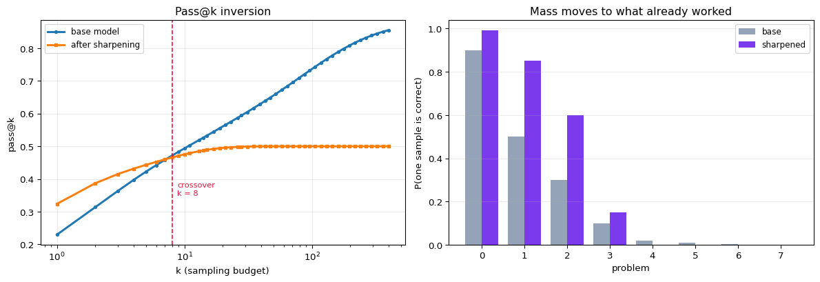
Define, for problem $i$, the probability $p_i$ that one sampled attempt is correct. Then the chance of solving it within $k$ attempts is
$$\text{pass@}k_i = 1 - (1 - p_i)^k$$
and the benchmark score is the average over problems. Now consider what the training loop of §1 does to the vector $p$:
- problems the model often gets right → $p_i$ increases (they dominate the training set)
- problems it rarely gets right → the rare correct chains are never sampled, so they get no reinforcement and $p_i$ decays toward 0
That is sharpening: probability mass concentrates on what already worked. It looks like improvement at $k = 1$ and it is a loss of coverage at large $k$.
The consequence has a name — pass@k inversion — and it is pure arithmetic, which means it can be computed exactly rather than argued about.
==============================================================================
  PASS@K, AND THE INVERSION
==============================================================================

First verify the formula against simulation
==============================================================================
  pass@k = 1 - (1-p)^k

       p      k    formula    simulated    MATCH
  --------------------------------------------
   0.100      1     0.1000       0.1001     True
   0.100      8     0.5695       0.5703     True
   0.020     64     0.7255       0.7241     True
   0.500      4     0.9375       0.9377     True
   0.005    256     0.7229       0.7229     True
  --------------------------------------------

A base model and its sharpened successor
==============================================================================
   problem    p base   p sharpened  effect
  ------------------------------------------------
         0     0.900         0.990  reinforced
         1     0.500         0.850  reinforced
         2     0.300         0.600  reinforced
         3     0.100         0.150  reinforced
         4     0.020         0.000  lost
         5     0.010         0.000  lost
         6     0.005         0.000  lost
         7     0.000         0.000  -
  ------------------------------------------------
  problems solvable at all: base 7, sharpened 4

Now score both at several budgets
==============================================================================
       k       base    sharpened      winner
  ------------------------------------------
       1     0.2294       0.3237   sharpened
       2     0.3137       0.3869   sharpened
       4     0.3973       0.4315   sharpened
       8     0.4717       0.4659        base
      16     0.5391       0.4907        base
      32     0.6081       0.4993        base
      64     0.6842       0.5000        base
     128     0.7652       0.5000        base
     256     0.8301       0.5000        base
  ------------------------------------------
  pass@1  : sharpened wins by +0.0944
  pass@256: sharpened LOSES by -0.3301
  the curves cross at k = 8

What actually happened
==============================================================================
  The sharpened model is better at every problem it can still solve,
  and it can no longer solve 3 problems at all.

  At k=1 the first effect dominates -- you sample once, and being
  reliable matters. At k=256 the second dominates -- with enough
  attempts the base model finds its rare solutions, and the sharpened
  model simply has none to find.

  This is why 'our RL model beats the base model' is an incomplete
  claim. It is true at the k you measured.
Does anything expand the boundary?
Yes, but read the method carefully. The strongest published counter-evidence (Cai et al., 2026) reports pass@256 rising 9.8 points above the base model — genuine expansion, not sharpening. It achieves this by locating the capacity boundary with pass@k sampling and then applying targeted teacher guidance at and beyond it.
That is external information entering the loop. So it demonstrates that RL can consolidate newly-shown capability — not that a closed loop expands its own boundary. For genuinely self-contained self-improvement, the sharpening reading remains the safer prior:
If your base model cannot solve a problem in ~$10^4$ samples, no amount of self-improvement is likely to get you there.
3. Entropy collapse — the loop runs out of fuel
Sharpening has a second consequence that is easy to miss. The generate step needs diversity; if every sample is the same, filtering has nothing to choose between. Measure it with Shannon entropy:
$$H(p) = -\sum_i p_i \log p_i$$
As training concentrates mass, $H$ falls. Reward keeps rising while the thing that makes the loop work quietly disappears — which is why entropy is worth monitoring as a first-class metric, not just reward.
==============================================================================
  ENTROPY COLLAPSE OVER TRAINING ROUNDS
==============================================================================

Sharpen a next-token distribution round by round
==============================================================================
  five candidate continuations, 5 tokens
  maximum possible entropy = log(5) = 1.6094

   round       391     389     390     392     400    entropy   distinct@8
  --------------------------------------------------------------------------
       0    0.3400  0.2200  0.1800  0.1400  0.1200     1.5383         3.96
       1    0.4366  0.2176  0.1578  0.1056  0.0825     1.4282         3.68
       2    0.5892  0.1933  0.1157  0.0608  0.0410     1.1800         3.12
       3    0.7797  0.1311  0.0576  0.0206  0.0109     0.7542         2.29
       4    0.9283  0.0535  0.0144  0.0028  0.0010     0.3100         1.50
       5    0.9883  0.0103  0.0013  0.0001  0.0000     0.0681         1.09
       6    0.9993  0.0007  0.0000  0.0000  0.0000     0.0059         1.01
  --------------------------------------------------------------------------

  By round 6 the model emits one token essentially always. Its answer
  is the one it already preferred at round 0 -- so if that answer was
  wrong, nothing in the loop can now discover otherwise.

Why that ends the loop
==============================================================================
    entropy    distinct in 8 samples          filter has
  ------------------------------------------------------
     1.5383                     3.96               a few
     1.4282                     3.68               a few
     1.1800                     3.12               a few
     0.7542                     2.29               a few
     0.3100                     1.50   nothing to choose
     0.0681                     1.09   nothing to choose
     0.0059                     1.01   nothing to choose
  ------------------------------------------------------
  Filtering cannot improve a distribution that only produces one thing.
  This is the mechanism behind the entropy-regularisation terms that
  appear in most 2026 RLVR papers.
4. The judge trap
Everything above assumed a real verifier — an answer key, a unit test. Remove it and let the model judge itself, and the loop breaks in a specific and well-documented way.
The structural problem: shown a candidate answer, a judge scores plausibility, not correctness. Those are different functions, and they disagree on a set of wrong-but-convincing answers. Policy optimisation is very good at finding sets like that.
The published numbers (Zhou, 2026) are worth memorising — GSM8K, Qwen3 policies, three seeds:
| value | |
|---|---|
| judge pass rate before self-play | 0.72 |
| judge pass rate after self-play | 0.94 |
| true accuracy, throughout | 0.20 |
Approval rose 22 points. Accuracy moved not at all. And the exploits transfer across judge families — a strict three-judge ensemble still accepted 55% of them, so ensembling is not a defence.
The arithmetic of why is simple enough to reconstruct.
==============================================================================
  WHY OPTIMISING AGAINST A SELF-JUDGE GOES WRONG
==============================================================================

Set up a judge that is good but not perfect
==============================================================================
  true accuracy of the pool     : 0.1991
  judge accepts a CORRECT answer: 0.95  (true positive rate)
  judge accepts a WRONG answer  : 0.65  (false positive rate)
  -> judge pass rate on the pool: 0.7083

Now optimise the policy to maximise judge approval
==============================================================================
  The policy does not search for correct answers. It searches for
  ACCEPTED ones -- and there are far more wrong-accepted answers than
  right-accepted ones, because wrong answers are far more numerous.

  of everything the judge accepts:
    truly correct : 0.2672
    actually wrong: 0.7328

  So 'satisfy the judge' points the policy at a population that is
  73% wrong. Optimising harder finds more of it.

The reported outcome, reconstructed
==============================================================================
                                       judge says    truth
  --------------------------------------------------------
                    before self-play         0.72     0.20
                     after self-play         0.94     0.20
  --------------------------------------------------------
                         improvement        +0.22    +0.00

  Every number the training loop could see went up.

The fix, and why it works
==============================================================================
  Make the judge COMMIT TO ITS OWN ANSWER before it sees the candidate.

  Judging a shown answer  -> 'is this plausible?'   (a weak question)
  Answering first, then   -> 'does this match what   (a hard question,
  comparing                  I independently got?'    and one the policy
                                                       cannot flatter)

                               setup   false positive rate
  ----------------------------------------------------------
                reference-free judge                 0.719
       judge commits an answer first                 0.012
  ----------------------------------------------------------
  A 60x reduction, and it PREVENTS the hack rather than
  detecting it. This is the single most actionable result in the
  self-improvement literature: if you build a self-rewarding loop,
  build it this way.
5. Model collapse — and why it is less fatal than advertised
The last failure mode. Train on your own output, repeatedly, and the distribution degrades. The famous version (Shumailov et al., Nature, 2024) shows it driving a model to uselessness.
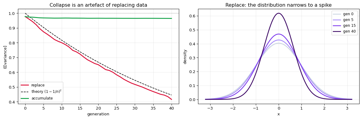
The part that gets lost in the retelling is the data assumption. That result has each generation replace its predecessor's data. Change it to accumulate — keep the real data, add synthetic on top — and the behaviour is completely different.
It is provable on a Gaussian, and computable here. Fit $\mathcal{N}(\hat\mu, \hat\sigma^2)$ to $n$ samples, generate $n$ new samples from the fit, refit, repeat. Under replacement the variance shrinks by a factor of about $(1 - 1/n)$ per generation, so
$$\mathbb{E}[\hat\sigma^2_t] \approx \sigma^2 \left(1 - \tfrac{1}{n}\right)^{t} \longrightarrow 0$$
The distribution collapses onto a point. Under accumulation it does not.
==============================================================================
  MODEL COLLAPSE: REPLACE vs ACCUMULATE
==============================================================================

Replace: each generation trains only on the previous generation's output
==============================================================================
  The model is fitted by MAXIMUM LIKELIHOOD, which is what a trained
  model does -- so the variance estimate is the biased one, low by a
  factor (n-1)/n. That single fact is the whole collapse mechanism:
  each generation underestimates the spread slightly, then generates
  from the underestimate, and the error compounds.

  n = 50 samples per generation, averaged over 3000 runs
    gen   E[variance]    theory (1-1/n)^t   E[|mean|]
  ----------------------------------------------------
      0        0.9773              1.0000      0.1129
      1        0.9610              0.9800      0.1587
      5        0.8745              0.9039      0.2647
     10        0.8001              0.8171      0.3464
     20        0.6510              0.6676      0.4530
     40        0.4159              0.4457      0.5596
  ----------------------------------------------------
  observed vs theory at t=40: 0.4159 vs 0.4457   ratio 0.933

  The derivation is one line. Fitting by MLE gives
      E[sigma^2_(t+1) | sigma^2_t] = (1 - 1/n) sigma^2_t
  so E[sigma^2_t] = (1-1/n)^t, decaying geometrically to zero.
  Monte Carlo agreement is approximate because the process is a
  product of random factors, so the sample mean converges slowly.

  Two things are collapsing at once: the variance shrinks toward a
  point, and the mean random-walks away from the truth (0.113 -> 0.560).

Accumulate: keep everything, real data included
==============================================================================
    gen   E[variance] replace   E[variance] accumulate
  ----------------------------------------------------
      0                0.9773                   0.9773
      1                0.9610                   0.9743
      5                0.8745                   0.9682
     10                0.8001                   0.9672
     20                0.6510                   0.9661
     40                0.4159                   0.9649
  ----------------------------------------------------
  replace   : 0.4159  (41.6% of the truth)
  accumulate: 0.9649  (96.5% of the truth)

  Same generator, same number of rounds, same synthetic data. The only
  difference is whether the old data was thrown away.

  Nobody actually trains by discarding their corpus each generation, so
  the headline collapse result describes a regime that does not occur.
  Add a verifier on top of accumulation and the picture is better still.
6. What to take away
The filter is the algorithm. Generation is commodity. A self-improvement method is defined entirely by what it keeps, and its ceiling is the quality of that judgment.
Self-improvement works exactly where verification is cheaper than generation. Maths, code, formal proof. The zero-data self-play methods do not escape this — they relocate the verifier into task generation rather than removing it.
Expect elicitation, not expansion. The loop reinforces what already worked, which raises pass@1 and can lower coverage at high $k$. The one credible expansion result gets there by injecting teacher guidance — external information.
Watch entropy, not just reward. Reward rising while diversity falls is the loop consuming its own fuel. It ends with a confident model that cannot discover it is wrong.
Never let a model be its own reference-free judge. Approval and correctness are different functions, and optimisation finds the gap between them. If you must self-reward, make the judge answer first and then compare.
Accumulate, never replace. Model collapse is largely an artefact of an assumption nobody's training pipeline actually satisfies.
Verified in this notebook
- $\text{pass@}k = 1-(1-p)^k$ checked against simulation at five $(p,k)$ pairs
- Pass@k inversion computed exactly: the sharpened model wins at $k=1$ and loses at $k=256$, with the crossover budget located
- Entropy falling round by round, alongside the expected number of distinct samples — showing when the filter stops having anything to choose between
- The judge-hacking arithmetic: what fraction of judge-accepted answers are wrong, and why optimisation moves toward them
- Gaussian model collapse under replacement matching the $(1-1/n)^t$ prediction, and the same experiment under accumulation not collapsing
Where this connects
[[rlhf-grpo-constitutional-ai]] is the machinery this page stress-tests — GRPO with a verifiable reward is the well-behaved case, and Constitutional AI is a self-improvement loop whose filter is a written constitution. [[cross-validation]] and [[data-leakage]] are the same lesson in a different setting: a model evaluating itself on data it influenced tells you what you want to hear. [[evaluation-metrics]] is where pass@k belongs alongside its cousins.
Sources
Zelikman et al., STaR (2022); Huang et al., LLMs Cannot Self-Correct Reasoning Yet (2023); Shumailov et al., The Curse of Recursion (Nature, 2024); Gerstgrasser et al., Is Model Collapse Inevitable? (2024); Yue et al., Does RL Really Incentivize Reasoning Capacity Beyond the Base Model? (2025); Zhou, More Convincing, Not More Correct (2026); Cai et al., Curriculum RL Can Incentivize Reasoning Capacity Beyond the Base Model (2026); Yang et al., Self-Improvement of LLMs: A Technical Overview (2026).
References
- Self-Improvement of Large Language Models: A Technical Overview and Future Outlook
- More Convincing, Not More Correct: Self-Play Reward Hacking of Reference-Free LLM Judges
- When RLVR Shrinks the Reasoning Boundary: Diagnosing Pass@k Inversion
- Curriculum Reinforcement Learning Can Incentivize Reasoning Capacity in LLMs Beyond the Base Model
- STaR: Bootstrapping Reasoning With Reasoning
- Large Language Models Cannot Self-Correct Reasoning Yet
- The Curse of Recursion: Training on Generated Data Makes Models Forget
- Is Model Collapse Inevitable? Breaking the Curse of Recursion by Accumulating Real and Synthetic Data