🛡 Support Vector Machine
Logistic regression finds a line that separates the classes. When several lines all achieve zero errors, nothing in its loss prefers one over another.
The support vector machine adds the missing criterion: pick the line with the widest margin. Formally, maximise the distance to the nearest point of either class:
$$\max_{\mathbf{w},b} \; \frac{2}{\lVert\mathbf{w}\rVert} \quad\text{subject to}\quad y_i(\mathbf{w}^\top\mathbf{x}_i + b) \ge 1$$
Two consequences follow, and both are visible in the numbers below:
- Only the points on the margin matter. Everything else could be deleted without changing the answer — those few points are the support vectors.
- The optimisation depends on the data only through inner products $\mathbf{x}_i^\top\mathbf{x}_j$. Replace that product with a kernel and the same algorithm draws curved boundaries in the original space without ever computing coordinates there.
Display helpers ready: banner, step, check, expand, show_matrix, show_matmul, show_elementwise.
1. The Data
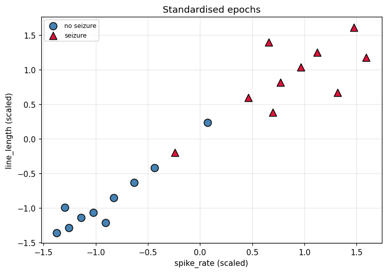
The same 20 EEG epochs as the Logistic Regression and KNN walkthroughs.
Features are standardised throughout. For an SVM this is not cosmetic: the margin is measured with a Euclidean norm, so unscaled features distort what "widest" means — exactly the problem shown in the KNN notebook.
20 epochs x 2 features, classes [10, 10]

    id   spike_rate   line_length   class         label
-------------------------------------------------------
  ep00          1.0          12.0       0    no seizure
  ep01          1.6          15.0       0    no seizure
  ep02          0.7          11.0       0    no seizure
  ep03          2.1          18.0       0    no seizure
  ep04          1.3          14.0       0    no seizure
  ep05          2.6          21.0       0    no seizure
  ep06          0.9          16.0       0    no seizure
  ep07          1.9          13.0       0    no seizure
  ep08          3.1          24.0       0    no seizure
  ep09          4.4          33.0       0    no seizure
  ep10          6.2          41.0       1       seizure
  ep11          7.1          47.0       1       seizure
  ep12          5.4          38.0       1       seizure
  ep13          8.0          52.0       1       seizure
  ep14          6.7          44.0       1       seizure
  ep15          5.9          49.0       1       seizure
  ep16          7.6          39.0       1       seizure
  ep17          6.0          35.0       1       seizure
  ep18          3.6          27.0       1       seizure
  ep19          8.3          46.0       1       seizure
-------------------------------------------------------

feature means : [ 4.22 29.75]
feature stds  : [ 2.564 13.794]

Note the scales: line_length spans ~41 while spike_rate spans ~8.
Any algorithm that measures DISTANCE will be dominated by the larger one
unless the features are scaled - that matters for KNN and SVM below.
labels recoded for SVM: [-1 -1 -1 -1 -1 -1 -1 -1 -1 -1  1  1  1  1  1  1  1  1  1  1]

The +/-1 convention is what makes the constraint y*(w.x + b) >= 1 work for
both classes with a single expression.
2. The Line, and What $\mathbf{w}$ and $b$ Actually Mean
Before any optimisation, be precise about the object being optimised. A straight boundary in two dimensions is written
$$w_1x_1 + w_2x_2 + b = 0 \qquad\text{or}\qquad \mathbf{w}^\top\mathbf{x} + b = 0$$
Two facts about this form do all the work later, and both are checkable:
$\mathbf{w}$ is perpendicular to the line. Take any two points $\mathbf{p}, \mathbf{q}$ that lie on the line. Both satisfy the equation, so subtracting gives $\mathbf{w}^\top(\mathbf{p} - \mathbf{q}) = 0$. The vector $\mathbf{p}-\mathbf{q}$ points along the line, and its dot product with $\mathbf{w}$ is zero — so $\mathbf{w}$ points straight across it. This is why $\mathbf{w}$ is called the normal vector, and it is the reason every distance on this page is measured in the direction of $\mathbf{w}$.
The sign of $\mathbf{w}^\top\mathbf{x}+b$ says which side you are on. Positive on one side, negative on the other, exactly zero on the line. That single number is called the decision value, and classification is nothing more than reading its sign.
$b$ does not change the direction of the line, only how far it sits from the origin. Changing $\mathbf{w}$ rotates the boundary; changing $b$ slides it.
==============================================================================
  THE LINE, AND WHAT w AND b MEAN
==============================================================================
  using 18 of 20 epochs (ep09 and ep18 held back until section 8)
  class -1: 9 epochs      class +1: 9 epochs

Fact 1: w is perpendicular to the line it defines
==============================================================================
  w = [0.6 0.8],  b = -0.1
  the line is  0.60*x1 + 0.80*x2 + (-0.10) = 0

  point p on the line = [-2.     1.625]   check w.p + b = +8.33e-17
  point q on the line = [ 2.    -1.375]   check w.q + b = +8.33e-17

  direction ALONG the line, p - q = [-4.  3.]
  w . (p - q) = (0.60)(-4.0000) + (0.80)(+3.0000) = +4.44e-16
  zero to floating point: True

  A zero dot product means a 90 degree angle. So w is normal to the line,
  and 'moving perpendicular to the boundary' means 'moving along w'.

Fact 2: the sign of w.x + b is the side, and classification is reading it
==============================================================================
    epoch        x1        x2     w.x + b    sign   true y  ok
  --------------------------------------------------------------
     ep00   -1.2560   -1.2867     -1.8830      -1       -1  yes
     ep02   -1.3730   -1.3592     -2.0112      -1       -1  yes
     ep04   -1.1390   -1.1418     -1.6968      -1       -1  yes
     ep06   -1.2950   -0.9968     -1.6744      -1       -1  yes
     ep08   -0.4369   -0.4168     -0.6956      -1       -1  yes
     ep11    1.1234    1.2505      1.5744      +1       +1  yes
     ep13    1.4744    1.6130      2.0750      +1       +1  yes
     ep15    0.6553    1.3955      1.4096      +1       +1  yes
     ep17    0.6943    0.3806      0.6211      +1       +1  yes
  --------------------------------------------------------------
  this hand-picked line classifies 18/18 correctly

  Note what is NOT here: no notion yet of a good line versus a barely
  adequate one. Any line with all signs correct scores the same. That gap
  is what the margin fills.
3. Distance to a Line, and Why It Is Measured Perpendicular
The margin is a distance, so the distance has to be pinned down exactly.
For a point $\mathbf{x}_0$ the perpendicular distance to the boundary is
$$d(\mathbf{x}_0) = \frac{\lvert \mathbf{w}^\top\mathbf{x}_0 + b\rvert}{\lVert\mathbf{w}\rVert}$$
The numerator is the decision value from section 2. Dividing by $\lVert\mathbf{w}\rVert$ converts it into an actual geometric length — without that division you could double $\mathbf{w}$ and appear to double every distance while the line has not moved at all.
Why perpendicular? Because the shortest path from a point to a line is the perpendicular one. Any other route reaches the line at an angle and therefore travels further. When we ask "how close is the nearest point to the boundary", we mean the shortest distance, so we mean the perpendicular one.
The cell below does not assert this. It walks along the line, measures the straight-line distance from a point to each spot, and shows the minimum falling exactly on the perpendicular foot.
==============================================================================
  DISTANCE TO A LINE, AND WHY PERPENDICULAR IS THE RIGHT ONE
==============================================================================
  w = [0.6 0.8],  ||w|| = sqrt(0.60^2 + 0.80^2) = 1.000000

Distance from epoch ep00 at [-1.256  -1.2867]
==============================================================================
  decision value  w.x0 + b = (0.60)(-1.2560) + (0.80)(-1.2867) + (-0.10) = -1.882994
  distance        |-1.882994| / 1.000000 = 1.882994

The perpendicular foot, computed explicitly
==============================================================================
  move from x0 along -w by (w.x0+b)/||w||^2:
    foot = x0 - (-1.882994/1.000000) * w = [-0.1262  0.2196]
    is the foot on the line?  w.foot + b = +1.80e-16   -> True
    ||x0 - foot|| = 1.882994
    formula gave  = 1.882994
    MATCH: True

Now walk along the line and measure. Is the perpendicular really shortest?
==============================================================================
           point on line   distance to x0
  ------------------------------------------
             [-2.5  2. ]         3.514294
         [-2.     1.625]         3.005298
           [-1.5   1.25]         2.548456
         [-1.     0.875]         2.176852
             [-0.5  0.5]         1.940101
           [0.    0.125]         1.889590
           [ 0.5  -0.25]         2.039205
         [ 1.    -0.625]         2.351045
             [ 1.5 -1. ]         2.770870
         [ 2.    -1.375]         3.257189
           [ 2.5  -1.75]         3.784453
  ------------------------------------------
  minimum over the walk : 1.889342
  perpendicular formula : 1.882994
  the closest sampled point is 0.1548
  away from the exact foot, which is just the sampling step.

  So 'perpendicular' is not a convention someone chose. It is where the
  distance function bottoms out.

Signed distance: one number carrying both side and closeness
==============================================================================
  Dropping the absolute value keeps the sign, and multiplying by the
  label y makes it positive exactly when the point is on its own side:

    epoch    y      w.x+b   signed dist    y * dist  meaning
  ------------------------------------------------------------------
     ep00   -1    -1.8830       -1.8830      1.8830  correct side
     ep01   -1    -1.5686       -1.5686      1.5686  correct side
     ep08   -1    -0.6956       -0.6956      0.6956  correct side
     ep10   +1     1.0158        1.0158      1.0158  correct side
     ep16   +1     1.2275        1.2275      1.2275  correct side
  ------------------------------------------------------------------
  The quantity y*(w.x+b) is called the FUNCTIONAL MARGIN, and
  y*(w.x+b)/||w|| the GEOMETRIC margin. Section 5 explains why the
  algorithm optimises the first while we care about the second.
4. Which Line Is Best? The max–min Rule
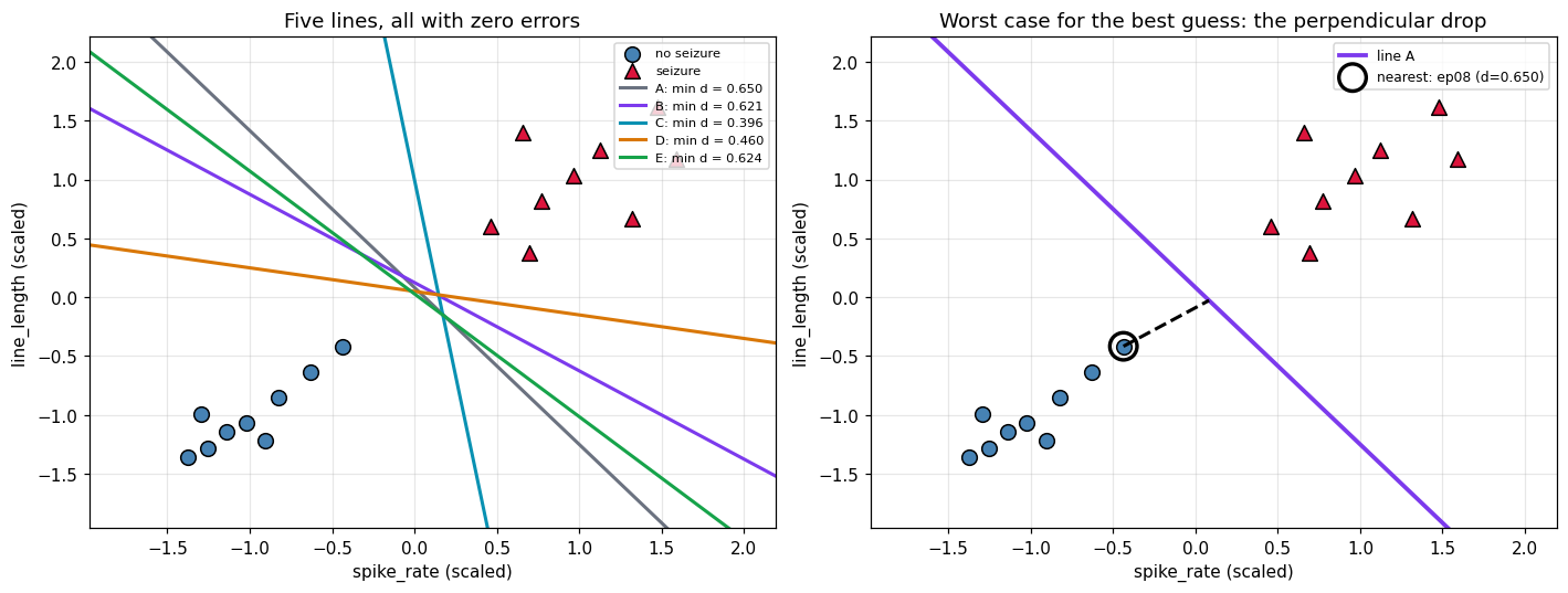
Now the actual question. Many lines classify every point correctly. Logistic regression has no preference between them; the SVM does.
For each candidate line, look at the nearest point to it — the worst case — and record that distance. Then choose the line whose worst case is the best:
$$\boxed{\;\max_{\mathbf{w},b}\;\Big[\;\min_i\; d(\mathbf{x}_i)\;\Big]\;}$$
Read it inside out: first find the closest point, then pick the line that pushes that closest point as far away as possible. It is a max of a min, and the two words are in that order for a reason — the goal is not the average distance, nor the sum, but the smallest one.
Why the worst case rather than the average? Because a line can sit far from most of the data and still shave past one point. That point is the one that will be misclassified when a slightly different sample arrives. Optimising the average would let the line trade safety on that point for distance from points that were never at risk.
The table below does this literally: several separating lines, and for each one the full list of distances collapsed to its minimum.
==============================================================================
  COMPARING CANDIDATE LINES BY THEIR NEAREST POINT
==============================================================================

Every candidate separates the data. That is not the question.
==============================================================================
   line                 w        b   separates?   errors
  ------------------------------------------------------
      A         [0.8 0.6]    -0.05         True        0
      B         [0.6 0.8]    -0.10         True        0
      C       [1.   0.15]    -0.15         True        0
      D         [0.2 1. ]    -0.05         True        0
      E       [0.72 0.69]    -0.02         True        0
  ------------------------------------------------------
  All five score zero errors. A loss that only counts mistakes cannot
  choose between them -- this is exactly the gap the margin fills.

Line B in full: the distance from every single epoch
==============================================================================
    epoch    y    distance
  --------------------------
     ep17   +1      0.6211   <- NEAREST
     ep12   +1      0.6546
     ep08   -1      0.6956
     ep05   -1      0.9866
     ep10   +1      1.0158
     ep16   +1      1.2275
     ep03   -1      1.2776
     ep14   +1      1.3068
     ep15   +1      1.4096
     ep01   -1      1.5686
     ep11   +1      1.5744
     ep07   -1      1.6144
     ep06   -1      1.6744
     ep04   -1      1.6968
     ep19   +1      1.7973
     ep00   -1      1.8830
     ep02   -1      2.0112
     ep13   +1      2.0750
  --------------------------
  min over all 18 epochs = 0.621054   (epoch ep17)
  mean distance          = 1.393902
  Only the first number matters to an SVM.

Collapse each candidate to its worst case, then rank
==============================================================================
   line   min distance   nearest epoch   mean distance
  ------------------------------------------------------
      A       0.649594            ep08        1.394313
      B       0.621054            ep17        1.393902
      C       0.395555            ep12        1.133355
      D       0.460332            ep17        1.170937
      E       0.623878            ep08        1.407974
  ------------------------------------------------------
  max over the min column -> line A, worst-case distance 0.649594

  Worth noticing: ranking by MEAN distance would pick line E, not A.
  The two criteria genuinely disagree, and the SVM takes the min.

None of these five is optimal - they were guessed
==============================================================================
  The true optimum is not on this list. Section 4 only shows what is being
  compared; sections 6 and 7 show how to actually find the best line,
  first by formula and then by iteration.
5. Three Parallel Lines, and the $\pm 1$ Convention
The max–min statement is correct but awkward to optimise, because $(\mathbf{w}, b)$ is not unique: multiplying both by any positive constant gives the identical line. Doubling $\mathbf{w}$ doubles every decision value while moving nothing.
The SVM removes that freedom by choosing a scale. Require the nearest points to produce a decision value of exactly $\pm 1$:
$$\mathbf{w}^\top\mathbf{x} + b = +1 \qquad \text{(upper margin line)}$$ $$\mathbf{w}^\top\mathbf{x} + b = \phantom{+}0 \qquad \text{(decision boundary)}$$ $$\mathbf{w}^\top\mathbf{x} + b = -1 \qquad \text{(lower margin line)}$$
All three are parallel — same $\mathbf{w}$, so the same normal direction, so the same slope. They differ only in offset.
This costs nothing, because it is a choice of units rather than a restriction on the line. What it buys is enormous: every point being on the correct side and outside the margin becomes a single clean inequality covering both classes,
$$y_i(\mathbf{w}^\top\mathbf{x}_i + b) \ge 1$$
and the points achieving equality — sitting exactly on a margin line — are the support vectors.
==============================================================================
  RESCALING CHANGES THE NUMBERS, NOT THE LINE
==============================================================================

Same line, three different (w, b) pairs
==============================================================================
   scale k                   w         b      w.x0+b    distance
  ------------------------------------------------------------
       0.5           [0.3 0.4]    -0.050     -0.9415    1.882994
       1.0           [0.6 0.8]    -0.100     -1.8830    1.882994
       2.0           [1.2 1.6]    -0.200     -3.7660    1.882994
       5.0             [3. 4.]    -0.500     -9.4150    1.882994
  ------------------------------------------------------------
  The decision value scales with k. The DISTANCE does not move at all,
  because the ||w|| in the denominator scales with it too.
  So (w, b) has one redundant degree of freedom, and we may spend it.

Spend it: rescale so the nearest point sits at exactly |w.x+b| = 1
==============================================================================
  smallest functional margin before : 0.621054
  rescale by k = 1/0.621054 = 1.610166
  smallest functional margin after  : 1.000000
  every point now satisfies y(w.x+b) >= 1 : True

With the scale fixed, the three lines have concrete meaning
==============================================================================
  w = [0.9661 1.2881],  b = -0.1610,  ||w|| = 1.610166

                    line                    equation   distance from boundary
  ----------------------------------------------------------------------------
            upper margin                w.x + b = +1                 0.621054
       decision boundary                w.x + b =  0                 0.000000
            lower margin                w.x + b = -1                 0.621054
  ----------------------------------------------------------------------------
  total width between the margin lines = 2/||w|| = 1.242108

Who is a support vector? Whoever achieves equality
==============================================================================
    epoch    y      w.x+b    y(w.x+b)  status
  ----------------------------------------------------
     ep17   +1     1.0000      1.0000  SUPPORT VECTOR (on the margin)
     ep12   +1     1.0540      1.0540  outside the margin
     ep08   -1    -1.1200      1.1200  outside the margin
     ep05   -1    -1.5886      1.5886  outside the margin
     ep10   +1     1.6356      1.6356  outside the margin
     ep16   +1     1.9765      1.9765  outside the margin
     ep03   -1    -2.0571      2.0571  outside the margin
     ep14   +1     2.1042      2.1042  outside the margin
     ep15   +1     2.2696      2.2696  outside the margin
     ep01   -1    -2.5257      2.5257  outside the margin
     ep11   +1     2.5351      2.5351  outside the margin
     ep07   -1    -2.5994      2.5994  outside the margin
     ep06   -1    -2.6961      2.6961  outside the margin
     ep04   -1    -2.7321      2.7321  outside the margin
     ep19   +1     2.8939      2.8939  outside the margin
     ep00   -1    -3.0319      3.0319  outside the margin
     ep02   -1    -3.2384      3.2384  outside the margin
     ep13   +1     3.3411      3.3411  outside the margin
  ----------------------------------------------------
  1 support vector(s): ['ep17']

  This line was only rescaled, not optimised -- so it touches the margin
  at whichever point happened to be nearest. After optimisation the
  margin lines are pushed apart until they are pinned from BOTH sides.
Why $1$? And why $\pm 1$ is not a distance
Two questions people get stuck on here, and they have different answers.
"Why 1 and not 5?" No reason. Any positive constant works. Requiring the nearest points to give $\pm 5$ describes exactly the same geometry — divide $\mathbf{w}$ and $b$ by 5 and you are back to $\pm 1$. The 1 is chosen because it makes the constraint read $y_i(\mathbf{w}^\top\mathbf{x}_i+b) \ge 1$ instead of $\ge 5$. It is a choice of units, like measuring in metres rather than centimetres.
"What if the classes are only 0.5 apart? How can the margin be 1?" This is the real confusion, and the answer is that it isn't. The numbers $\pm 1$ are values of the decision function $f(\mathbf{x}) = \mathbf{w}^\top\mathbf{x}+b$, not lengths on the plot. The actual geometric gap is
$$\text{margin} = \frac{2}{\lVert\mathbf{w}\rVert}$$
and if the classes really are 0.5 apart, the optimiser produces $\lVert\mathbf{w}\rVert = 4$, so $2/4 = 0.5$. The decision values stay at $\pm 1$; $\lVert\mathbf{w}\rVert$ absorbs the geometry. Nothing is being asserted about how far apart your classes are.
A trap worth naming
It is tempting to conclude: "minimising $\lVert\mathbf{w}\rVert$ widens the margin, so take $\mathbf{w} = (4,2)$, halve it to $(1,0.5)$, and the margin grows four-fold."
That is false, and the reason matters. Scaling $\mathbf{w}$ and $b$ together gives the same line — section 5 opened by showing exactly that. If the line has not moved, no distance to it can have changed.
What goes wrong is that $2/\lVert\mathbf{w}\rVert$ is only the margin when the scale is fixed by the constraint. Divorced from that, it is just a number. The quantity that is genuinely scale-free is
$$\text{geometric margin} = \min_i \frac{y_i\,(\mathbf{w}^\top\mathbf{x}_i+b)}{\lVert\mathbf{w}\rVert}$$
and the cell below shows it staying stubbornly constant while $2/\lVert\mathbf{w}\rVert$ swings by a factor of eight.
Minimising $\lVert\mathbf{w}\rVert$ only widens the margin subject to $y_i(\mathbf{w}^\top\mathbf{x}_i+b) \ge 1$. Drop the constraint and the honest answer is $\mathbf{w} = \mathbf{0}$, an infinite margin and no classifier at all.
==============================================================================
  2/||w|| IS NOT THE MARGIN UNLESS THE SCALE IS PINNED
==============================================================================

Rescale the SAME line and watch the two quantities disagree
==============================================================================
       k     ||kw||    2/||kw||   min y*f(x)   geometric margin
  --------------------------------------------------------------
    0.25     0.4025      4.9684       0.2500           0.621054
    0.50     0.8051      2.4842       0.5000           0.621054
    1.00     1.6102      1.2421       1.0000           0.621054
    2.00     3.2203      0.6211       2.0000           0.621054
    4.00     6.4407      0.3105       4.0000           0.621054
  --------------------------------------------------------------
  Column 3 changes by a factor of 16 across these rows.
  Column 5 does not move at all -- because the line did not move.

  Every row above is the SAME boundary. Check it: the predictions are
  identical for every k -> True

So the 'shrink w to widen the margin' shortcut is wrong
==============================================================================
  line A: w = [4. 2.], b = -1.00   ||w|| = 4.4721   2/||w|| = 0.4472
  line B: w = [1.  0.5], b = -0.25   ||w|| = 1.1180   2/||w|| = 1.7889

  2/||w|| suggests line B has a 4x wider margin. But:
    a point on line A: [0.  0.5]   on line B? w_B.x + b_B = +0.00e+00
    a point on line A: [ 1.  -1.5]   on line B? w_B.x + b_B = +0.00e+00
    -> A and B are the SAME LINE. The margin cannot have changed.

  geometric margin of A = 0.455535
  geometric margin of B = 0.455535
  equal: True

What DOES change the margin: a different direction
==============================================================================
  Rotating w is the only way to move the boundary. Same points,
  each direction normalised so the nearest point sits at exactly 1:

         direction w   ||w|| after   true margin 2/||w||
  --------------------------------------------------------
             [1. 0.]        2.2293              0.897138
           [0.7 0.7]        1.4793              1.352014
           [0.6 0.8]        1.5190              1.316641
       [0.708 0.706]        1.4794              1.351928  <- joins the class means
  --------------------------------------------------------
  These are genuinely different margins, because these are genuinely
  different lines. That is the comparison section 4 was making, and
  it is the one minimising ||w||^2 under the constraint carries out.
6. Margin, and Why It Is $2/\lVert\mathbf{w}\rVert$
The boundary is $\mathbf{w}^\top\mathbf{x} + b = 0$. Fix the scale by requiring the closest points of each class to satisfy $\mathbf{w}^\top\mathbf{x} + b = \pm 1$ — this costs nothing, since $(\mathbf{w}, b)$ can always be rescaled.
The signed distance from a point to the hyperplane is
$$\text{distance} = \frac{\mathbf{w}^\top\mathbf{x} + b}{\lVert\mathbf{w}\rVert}$$
so the two margin planes sit at $\pm 1/\lVert\mathbf{w}\rVert$, and the gap between them is
$$\text{margin} = \frac{2}{\lVert\mathbf{w}\rVert}$$
Maximising the margin is therefore minimising $\lVert\mathbf{w}\rVert$ — which is why the SVM objective looks like a regularisation term with constraints attached.
w = [0.8873 0.8112]     b = +0.075223
||w|| = sqrt(0.8873^2 + 0.8112^2) = 1.202211
margin = 2 / ||w|| = 2 / 1.202211 = 1.663602

    id     w.x + b     y    y(w.x+b)   dist to plane            status
------------------------------------------------------------------------
  ep18    -0.30107     1    -0.30107        -0.25043     MISCLASSIFIED
  ep09     0.32864    -1    -0.32864         0.27336     MISCLASSIFIED
  ep08    -0.65054    -1     0.65054        -0.54112    support vector
  ep12     0.96876     1     0.96876         0.80582    support vector
  ep17     1.00000     1     1.00000         0.83180    support vector
  ep05    -1.00000    -1     1.00000        -0.83180    support vector
  ep03    -1.34946    -1     1.34946        -1.12249    safely outside
  ep10     1.42205     1     1.42205         1.18287    safely outside
  ep01    -1.69893    -1     1.69893        -1.41317    safely outside
  ep07    -1.71271    -1     1.71271        -1.42464    safely outside
  ep14     1.77152     1     1.77152         1.47355    safely outside
  ep15     1.78868     1     1.78868         1.48782    safely outside
  ep16     1.78897     1     1.78897         1.48807    safely outside
  ep04    -1.86156    -1     1.86156        -1.54845    safely outside
  ep06    -1.88239    -1     1.88239        -1.56577    safely outside
  ep00    -2.08300    -1     2.08300        -1.73264    safely outside
  ep11     2.08637     1     2.08637         1.73545    safely outside
  ep02    -2.24564    -1     2.24564        -1.86792    safely outside
  ep19     2.44288     1     2.44288         2.03199    safely outside
  ep13     2.69189     1     2.69189         2.23912    safely outside
------------------------------------------------------------------------

support vectors found by sklearn: ['ep05', 'ep08', 'ep09', 'ep12', 'ep17', 'ep18']
that is 6 of 20 points - the other 14 do not affect the solution at all.
Deleting the non-support vectors changes nothing
This is the claim worth testing directly: refit the SVM using only the support vectors and the boundary should be identical.
trained on all 20 points   : w = [0.8873 0.8112], b = +0.075223
trained on 6 support vectors: w = [0.8873 0.8112], b = +0.075223

same w? True
same b? True
same predictions on all 20 points? True

now move every NON-support vector 2 units further from the boundary:
   w before [0.8873 0.8112]  ->  after [0.8873 0.8112]
   unchanged? True

That is the defining property of an SVM: the solution is determined by a
handful of boundary cases, not by the bulk of the data.
7. Watching the Boundary Being Learned
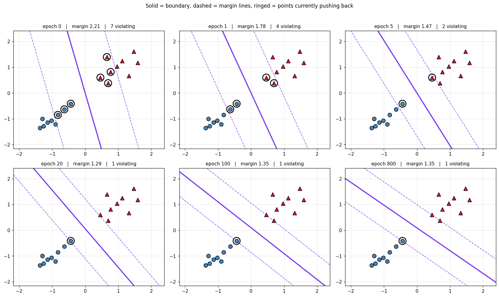
Section 6 gave the objective. This section watches it being solved, one update at a time, because that is where the algorithm stops being a formula and starts being something you can picture.
Production solvers use SMO or a quadratic programming routine. Those are efficient and completely opaque. What follows instead is subgradient descent on the hinge loss, which finds essentially the same boundary while letting every single update be inspected:
$$J(\mathbf{w}, b) \;=\; \underbrace{\lambda\lVert\mathbf{w}\rVert^2}_{\text{widen the margin}} \;+\; \underbrace{\frac{1}{n}\sum_i \max\big(0,\; 1 - y_i(\mathbf{w}^\top\mathbf{x}_i + b)\big)}_{\text{punish anything inside the margin}}$$
The whole algorithm turns on one test, evaluated for each point:
$$y_i(\mathbf{w}^\top\mathbf{x}_i + b) \;\ge\; 1\;?$$
- Satisfied — the point is on the right side and outside the margin. It has no complaint. Only the regularisation term acts, shrinking $\mathbf{w}$, which widens the margin: $\mathbf{w} \leftarrow \mathbf{w} - \eta\,(2\lambda\mathbf{w})$
- Violated — the point is misclassified, or correct but sitting inside the margin. It pushes back: $\mathbf{w} \leftarrow \mathbf{w} - \eta\,(2\lambda\mathbf{w} - y_i\mathbf{x}_i)$ and $b \leftarrow b + \eta\, y_i$
Read the violated case geometrically. The term $+\eta\,y_i\mathbf{x}_i$ moves $\mathbf{w}$ toward that point's own class direction, rotating the boundary away from it; and the $b$ update slides the line in the same sense. The point that complains is the point that moves the line.
Notice what this means: a point outside the margin never rotates the boundary. Only violators do. That is the mechanism behind "only support vectors matter", appearing here as a property of the update rule rather than as an assertion.
==============================================================================
  THE DECISION TEST, EVALUATED BY HAND
==============================================================================
  starting w = [0.882  0.2001],  b = 0.0000
  learning rate eta = 0.05,  regularisation lambda = 0.01

What the test says about each epoch, before any update
==============================================================================
    epoch    y      w.x+b    y(w.x+b)   >= 1?  verdict
  --------------------------------------------------------------------
     ep00   -1    -1.3653      1.3653    True  content, outside the margin
     ep01   -1    -1.1153      1.1153    True  content, outside the margin
     ep02   -1    -1.4830      1.4830    True  content, outside the margin
     ep03   -1    -0.8998      0.8998   False  correct side, INSIDE the margin
     ep04   -1    -1.2330      1.2330    True  content, outside the margin
     ep05   -1    -0.6843      0.6843   False  correct side, INSIDE the margin
     ep06   -1    -1.3417      1.3417    True  content, outside the margin
     ep07   -1    -1.0411      1.0411    True  content, outside the margin
     ep08   -1    -0.4687      0.4687   False  correct side, INSIDE the margin
     ep10   +1     0.8444      0.8444   False  correct side, INSIDE the margin
     ep11   +1     1.2410      1.2410    True  content, outside the margin
     ep12   +1     0.5256      0.5256   False  correct side, INSIDE the margin
     ep13   +1     1.6232      1.6232    True  content, outside the margin
     ep14   +1     1.0599      1.0599    True  content, outside the margin
     ep15   +1     0.8572      0.8572   False  correct side, INSIDE the margin
     ep16   +1     1.2970      1.2970    True  content, outside the margin
     ep17   +1     0.6885      0.6885   False  correct side, INSIDE the margin
     ep19   +1     1.6394      1.6394    True  content, outside the margin
  --------------------------------------------------------------------
  11 satisfied, 7 violating  -> 7 points will push the line this epoch
==============================================================================
  THE FIRST FIVE UPDATES, WRITTEN OUT IN FULL
==============================================================================

  update 1: epoch ep00, x = [-1.256  -1.2867], y = -1
    w.x + b   = (+0.8820)(-1.2560) + (+0.2001)(-1.2867) + (+0.0000) = -1.365269
    y(w.x+b)  = (-1)(-1.365269) = +1.365269   >= 1  SATISFIED
    rule: w <- w - eta*(2*lambda*w)          [only shrink w]
    w: [0.882  0.2001] -> [0.8811 0.1999]   (moved 0.000904)
    b: +0.000000 -> +0.000000   (moved 0.000000)

  update 2: epoch ep01, x = [-1.022  -1.0693], y = -1
    w.x + b   = (+0.8811)(-1.0220) + (+0.1999)(-1.0693) + (+0.0000) = -1.114215
    y(w.x+b)  = (-1)(-1.114215) = +1.114215   >= 1  SATISFIED
    rule: w <- w - eta*(2*lambda*w)          [only shrink w]
    w: [0.8811 0.1999] -> [0.8803 0.1997]   (moved 0.000904)
    b: +0.000000 -> +0.000000   (moved 0.000000)

  update 3: epoch ep02, x = [-1.373  -1.3592], y = -1
    w.x + b   = (+0.8803)(-1.3730) + (+0.1997)(-1.3592) + (+0.0000) = -1.480022
    y(w.x+b)  = (-1)(-1.480022) = +1.480022   >= 1  SATISFIED
    rule: w <- w - eta*(2*lambda*w)          [only shrink w]
    w: [0.8803 0.1997] -> [0.8794 0.1995]   (moved 0.000903)
    b: +0.000000 -> +0.000000   (moved 0.000000)

  update 4: epoch ep03, x = [-0.8269 -0.8518], y = -1
    w.x + b   = (+0.8794)(-0.8269) + (+0.1995)(-0.8518) + (+0.0000) = -0.897100
    y(w.x+b)  = (-1)(-0.897100) = +0.897100   <  1  VIOLATED
    rule: w <- w - eta*(2*lambda*w - y*x)    [rotate toward this point]
          b <- b + eta*y
    w: [0.8794 0.1995] -> [0.9198 0.2419]   (moved 0.058605)
    b: +0.000000 -> -0.050000   (moved 0.050000)

  update 5: epoch ep04, x = [-1.139  -1.1418], y = -1
    w.x + b   = (+0.9198)(-1.1390) + (+0.2419)(-1.1418) + (-0.0500) = -1.373843
    y(w.x+b)  = (-1)(-1.373843) = +1.373843   >= 1  SATISFIED
    rule: w <- w - eta*(2*lambda*w)          [only shrink w]
    w: [0.9198 0.2419] -> [0.9189 0.2416]   (moved 0.000951)
    b: -0.050000 -> -0.050000   (moved 0.000000)

  Compare the two rules. A satisfied point changes w by a whisper and
  leaves b untouched. A violated point drags both. Over an epoch, the
  boundary is steered almost entirely by the points nearest to it.
==============================================================================
  TRAINING, WITH A SNAPSHOT AT EVERY CHECKPOINT
==============================================================================

What changes from epoch to epoch
==============================================================================
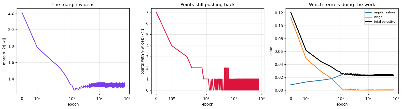
   epoch         w1         w2          b     ||w||   margin 2/||w||   violators   objective
  ----------------------------------------------------------------------------------------
       0     0.8820     0.2001     0.0000    0.9044           2.2113           7      0.1210
       1     1.0558     0.3797    -0.0000    1.1220           1.7826           4      0.0616
       5     1.2182     0.5972    -0.0000    1.3567           1.4741           2      0.0351
      20     1.2921     0.8629    -0.0500    1.5537           1.2872           1      0.0256
     100     1.0481     1.0430    -0.1000    1.4787           1.3526           1      0.0223
     800     0.9813     1.1103    -0.1000    1.4818           1.3497           1      0.0224
  ----------------------------------------------------------------------------------------
  Read the margin column together with the violator column, because
  2/||w|| is only a MARGIN once the constraints actually hold.

  Epoch 0 shows 2/||w|| = 2.2113, the largest figure in the table --
  and 7 points sitting between the margin lines. Wide lines with
  points inside them are not a margin, they are a meaningless number.

  So the trajectory has two phases:
    epochs 0-20   pushing points OUT of the margin. Doing that requires
                  a bigger ||w||, so the nominal margin FALLS
                  (2.2113 -> 1.2872) while the violator count drops 7 -> 1.
    epochs 20+    constraints essentially met, so the figure now means
                  what it says -- and regularisation widens it back
                  (1.2872 -> 1.3526).

  The second phase is minimising ||w||^2 doing its job. The first phase
  is the constraints being satisfied in the first place.

Where the objective goes
==============================================================================
   epoch    reg term    hinge term       total
  --------------------------------------------
       0      0.0082        0.1129      0.1210
       1      0.0126        0.0490      0.0616
       5      0.0184        0.0167      0.0351
      20      0.0241        0.0014      0.0256
     100      0.0219        0.0004      0.0223
     800      0.0220        0.0005      0.0224
  --------------------------------------------
  At epoch 0 the hinge term is 0.1129 against a regularisation term of
  0.0082 -- it is 14x larger, so essentially all of the
  gradient is the misclassified points shouting.

  By epoch 20 the hinge term has collapsed to 0.0014 and the two have
  swapped places. From there the regularisation term is the only one
  still doing anything, and what it does is shrink ||w||.

  This is why the total objective keeps falling after the last
  misclassification is gone: the constraints are satisfied, and the
  optimiser is still buying margin.

Final state
==============================================================================
  w = [0.9813 1.1103],  b = -0.100000
  ||w|| = 1.481773   margin = 2/||w|| = 1.349735
  all points satisfy y(w.x+b) >= 1 (to 1e-2): True
  training errors: 0/18

  Note the table above ends with 1 'violator'. That is ep08 at
  y(w.x+b) = 0.9915 -- a support vector sitting a hair under 1.0,
  not a misclassification. Training errors are 0. A strict
  'y(w.x+b) < 1' test counts points that are exactly ON the margin.

  points closest to the margin (3):
       ep08  y = -1   y(w.x+b) = 0.9915
       ep12  y = +1   y(w.x+b) = 1.0157
       ep17  y = +1   y(w.x+b) = 1.0039
Does the hand-rolled loop agree with a real solver?
The loop above is a teaching device. If it lands somewhere different from a proper QP solver, then watching it would teach the wrong thing — so the comparison below is the point, not a formality.
The two will not match to machine precision, and should not be expected to: subgradient descent with a fixed step size converges to a neighbourhood of the optimum rather than onto it, and the $\lambda$ used here corresponds to a particular $C$ in scikit-learn's parameterisation. What matters is that the boundary lands in the same place and picks out the same support vectors.
==============================================================================
  HAND-ROLLED SUBGRADIENT DESCENT vs A REAL QP SOLVER
==============================================================================

Parameters
==============================================================================
  lambda = 0.01 over n = 18 points corresponds to C = 1/(2*lambda*n) = 2.7778

                            w1          w2           b      ||w||     margin
  ------------------------------------------------------------------------
  gradient descent      0.9813      1.1103     -0.1000     1.4818     1.3497
       sklearn SVC      1.0055      1.0818     -0.1098     1.4769     1.3542
  ------------------------------------------------------------------------

Do they describe the same line?
==============================================================================
  angle between the two normal vectors = 1.438 degrees
  (0 would mean exactly parallel boundaries)

  identical predictions on 18/18 epochs
  training errors -- ours: 0,  sklearn: 0

Do they choose the same support vectors?
==============================================================================
  ours    : ['ep08', 'ep12', 'ep17']
  sklearn : ['ep08', 'ep12', 'ep17']
  overlap : ['ep08', 'ep12', 'ep17']
  identical set: True

  The boundary and the support vectors agree. The loop is a faithful,
  slower picture of what the solver computes in one shot.
What to carry forward from section 7
- The whole algorithm is one test, $y_i(\mathbf{w}^\top\mathbf{x}_i+b) \ge 1$, applied point by point. Everything else is bookkeeping around it.
- A point that passes the test contributes nothing but shrinkage. It cannot rotate the boundary. This is "only support vectors matter", derived rather than asserted.
- The two terms take turns: the hinge term dominates early, dragging misclassified points to the right side; the regularisation term takes over once they are, quietly widening the margin.
- $2/\lVert\mathbf{w}\rVert$ is only a margin once the constraints hold. Early on it is at its largest precisely because points are still sitting inside it, so it has to fall before it can rise. Read it next to the violator count or it will mislead you.
One honest caveat: real SVM solvers do not work this way. SMO and quadratic programming exploit the convexity of the problem to jump to the optimum instead of walking to it, and they solve the dual form of section 9 rather than this one. The picture above is faithful to the objective, not to the method — which is exactly the trade worth making while learning what the objective means.
8. Soft Margin and $C$
Sections 2-7 held back epochs ep09 and ep18 so that a separating line
existed at all. They come back now — and the whole point of this section
is that the SVM no longer needs them to be separable.
Our data is not separable — two epochs sit on the wrong side. A hard margin has no feasible solution at all, so slack variables $\xi_i \ge 0$ allow violations at a price:
$$\min_{\mathbf{w},b,\xi} \;\; \frac{1}{2}\lVert\mathbf{w}\rVert^2 + C\sum_i \xi_i \qquad\text{s.t.}\qquad y_i(\mathbf{w}^\top\mathbf{x}_i+b) \ge 1 - \xi_i$$
Equivalently, in unconstrained form with the hinge loss:
$$\min_{\mathbf{w},b}\;\; \frac{1}{2}\lVert\mathbf{w}\rVert^2 + C\sum_i \max\big(0,\; 1 - y_i(\mathbf{w}^\top\mathbf{x}_i + b)\big)$$
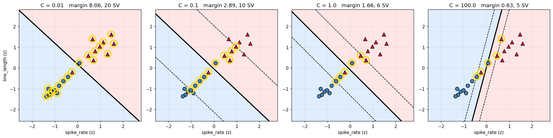
$C$ sets the exchange rate between margin width and violations:
- small $C$ — violations are cheap, so the margin grows wide and more points sit inside it
- large $C$ — violations are expensive, so the margin narrows to avoid them (approaching a hard margin)
C      ||w||     margin    #SV   sum slack   train acc    objective
------------------------------------------------------------------------
    0.01     0.2482     8.0578     20     13.8393      0.9000       0.1692
    0.10     0.6917     2.8914     10      4.6859      0.9000       0.7078
    1.00     1.2022     1.6636      6      3.0104      0.9000       3.7331
   10.00     1.5731     1.2714      4      2.7568      0.9000      28.8058
  100.00     3.1708     0.6307      5      2.6343      0.9000     268.4573
 1000.00     3.1749     0.6299      5      2.6346      0.9000    2639.6695
------------------------------------------------------------------------

As C grows the margin shrinks, the slack shrinks, and fewer points are
support vectors. Small C is the more regularised model.


hinge loss at C = 1, per point:

    id    y(w.x+b)      hinge                       meaning
------------------------------------------------------------
  ep09    -0.32864    1.32864             on the wrong side
  ep18    -0.30107    1.30107             on the wrong side
  ep08     0.65054    0.34946        inside margin, correct
  ep12     0.96876    0.03124        inside margin, correct
  ep04     1.86156    0.00000       outside margin, no cost
  ep01     1.69893    0.00000       outside margin, no cost
  ep02     2.24564    0.00000       outside margin, no cost
  ep00     2.08300    0.00000       outside margin, no cost
  ep07     1.71271    0.00000       outside margin, no cost
  ep06     1.88239    0.00000       outside margin, no cost
  ep05     1.00000    0.00000       outside margin, no cost
  ep10     1.42205    0.00000       outside margin, no cost
  ep11     2.08637    0.00000       outside margin, no cost
  ep13     2.69189    0.00000       outside margin, no cost
  ep14     1.77152    0.00000       outside margin, no cost
  ep03     1.34946    0.00000       outside margin, no cost
  ep15     1.78868    0.00000       outside margin, no cost
  ep16     1.78897    0.00000       outside margin, no cost
  ep17     1.00000    0.00000       outside margin, no cost
  ep19     2.44288    0.00000       outside margin, no cost
------------------------------------------------------------

total hinge = 3.010412
Gold circles are support vectors. Dashed lines are the margin boundaries.
Small C: wide margin, many support vectors, some violations tolerated.
Large C: narrow margin, few support vectors, violations avoided.
9. The Dual, and Where Kernels Come From
Introducing Lagrange multipliers $\alpha_i \ge 0$ for the constraints and eliminating $\mathbf{w}$ and $b$ gives the dual problem:
$$\max_{\alpha} \;\; \sum_i \alpha_i - \frac{1}{2}\sum_{i,j}\alpha_i\alpha_j y_i y_j \,\mathbf{x}_i^\top\mathbf{x}_j \qquad\text{s.t.}\qquad 0 \le \alpha_i \le C, \;\; \sum_i \alpha_i y_i = 0$$
and the solution is recovered as
$$\mathbf{w} = \sum_i \alpha_i y_i \mathbf{x}_i$$
Two things are now visible that were hidden in the original form:
- $\alpha_i = 0$ for every non-support vector. The sum runs only over the few points on or inside the margin.
- The data appears only as $\mathbf{x}_i^\top\mathbf{x}_j$. Nothing else. Replace that inner product with any valid kernel $K(\mathbf{x}_i,\mathbf{x}_j)$ and the algorithm is unchanged — this is the kernel trick.
sklearn returns 6 dual coefficients (alpha_i * y_i):

    id     y      alpha*y       alpha   at bound C?
--------------------------------------------------
  ep05    -1    -0.227861    0.227861            no
  ep08    -1    -1.000000    1.000000     yes (C=1)
  ep09    -1    -1.000000    1.000000     yes (C=1)
  ep12     1     1.000000    1.000000     yes (C=1)
  ep17     1     0.227861    0.227861            no
  ep18     1     1.000000    1.000000     yes (C=1)
--------------------------------------------------

constraint check: sum of alpha_i * y_i = +0.000e+00   (must be 0): True

recovering w from the dual:  w = sum_i alpha_i y_i x_i

   w[0] (spike_rate):
      (-0.2279)*(-0.6319) + (-1.0000)*(-0.4369) + (-1.0000)*(+0.0702) + (+1.0000)*(+0.4603) + (+0.2279)*(+0.6943) + (+1.0000)*(-0.2418)
      = +0.887281   |  sklearn: +0.887281   MATCH: True
   w[1] (line_length):
      (-0.2279)*(-0.6343) + (-1.0000)*(-0.4168) + (-1.0000)*(+0.2356) + (+1.0000)*(+0.5981) + (+0.2279)*(+0.3806) + (+1.0000)*(-0.1994)
      = +0.811199   |  sklearn: +0.811199   MATCH: True

full w MATCH: True

Every non-support vector has alpha = 0 and contributes nothing to this sum.
10. Kernels
A kernel computes an inner product in some feature space $\phi$ without ever building $\phi(\mathbf{x})$:
$$K(\mathbf{a},\mathbf{b}) = \phi(\mathbf{a})^\top\phi(\mathbf{b})$$
| Kernel | Formula | Feature space |
|---|---|---|
| Linear | $\mathbf{a}^\top\mathbf{b}$ | the original one |
| Polynomial | $(\gamma\,\mathbf{a}^\top\mathbf{b} + r)^d$ | all monomials up to degree $d$ |
| RBF / Gaussian | $\exp(-\gamma\lVert\mathbf{a}-\mathbf{b}\rVert^2)$ | infinite-dimensional |
The RBF case is the striking one: an infinite-dimensional feature map, evaluated in two arithmetic operations. The explicit expansion below shows why the polynomial kernel works, and by extension why the trick is legitimate.
take two epochs:  a = ep00 = [-1.256  -1.2867]
                  b = ep10 = [0.7723 0.8155]

POLYNOMIAL kernel, degree 2, gamma = 1, r = 1
------------------------------------------------------------
   K(a,b) = (a.b + 1)^2 = (-2.019426 + 1)^2 = 1.039229

   the explicit 6-dim map phi(x) = [1, sqrt2*x1, sqrt2*x2, x1^2, x2^2, sqrt2*x1*x2]
   phi(a) = [ 1.     -1.7762 -1.8197  1.5775  1.6557  2.2856]
   phi(b) = [1.     1.0922 1.1534 0.5965 0.6651 0.8908]

   phi(a).phi(b) = (+1.0000)*(+1.0000) + (-1.7762)*(+1.0922) + (-1.8197)*(+1.1534) +
      (+1.5775)*(+0.5965) + (+1.6557)*(+0.6651) + (+2.2856)*(+0.8908)
                 = 1.039229
   K(a,b)        = 1.039229
   MATCH: True

   The kernel computed in 2 operations what the explicit map needed 6
   dimensions for. In degree 3 with 10 features the map has 286 terms;
   the kernel is still one dot product and one power.

RBF kernel, gamma = 0.5
------------------------------------------------------------
   ||a - b||^2 = (-2.0283)*(-2.0283) + (-2.1023)*(-2.1023)
               = 8.533677
   K(a,b) = exp(-0.5 * 8.533677) = 0.01402605

   K depends ONLY on the distance, so it acts as a similarity that decays
   with separation. K(x,x) = 1 always, and K -> 0 for distant points.
RBF kernel matrix (first 6 epochs) (6, 6) =
                   ep00      ep01      ep02      ep03      ep04      ep05
         ep00 |  1.00000   0.95025   0.99057   0.82974   0.98279   0.66526
         ep01 |  0.95025   1.00000   0.90153   0.95823   0.99057   0.84310
         ep02 |  0.99057   0.90153   1.00000   0.75741   0.95025   0.58427
         ep03 |  0.82974   0.95823   0.75741   1.00000   0.91327   0.95823
         ep04 |  0.98279   0.99057   0.95025   0.91327   1.00000   0.77312
         ep05 |  0.66526   0.84310   0.58427   0.95823   0.77312   1.00000

   diagonal is all 1 (a point is maximally similar to itself): True
   symmetric: True
   smallest eigenvalue = 7.650e-08  -> positive semi-definite: True

   Positive semi-definiteness (Mercer's condition) is exactly what
   guarantees some feature space phi exists for this kernel.
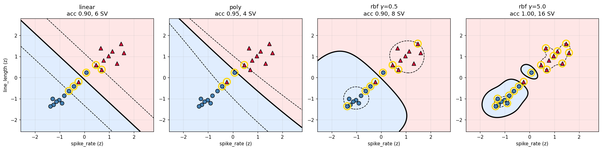
kernel   train acc    #SV
------------------------------------------
                linear      0.9000      6
                  poly      0.9500      4
         rbf gamma=0.5      0.9000      8
         rbf gamma=5.0      1.0000     16
------------------------------------------

gamma = 5 reaches 100% training accuracy by wrapping tight bubbles around
the two awkward epochs. That is memorisation, not generalisation - the
classic RBF failure mode when gamma is too large.
Seeing the lift: 2-D $\to$ 3-D on data no line can separate
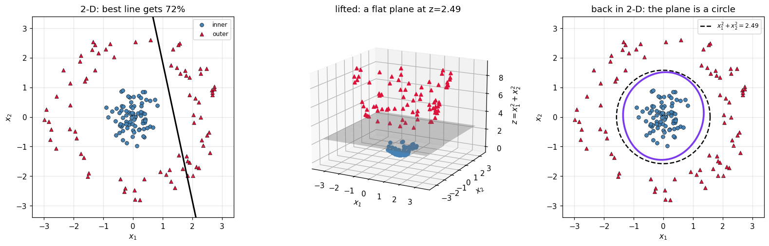
The kernel table above is abstract. Here is the concrete picture behind it, on the standard example: one class in a disc, the other in a ring around it.
No straight line separates these. Not a badly-chosen one — none exists. A linear SVM still reaches about 72% by slicing off one side of the ring, so the tell is not a score near chance; it is that the score cannot reach 100% however hard you fit. Both classes share a centre, so every half-plane containing the disc also swallows part of the ring.
Now add a third coordinate that measures distance from the centre:
$$\phi(x_1, x_2) = \big(x_1,\; x_2,\; x_1^2 + x_2^2\big)$$
Inner points get a small third coordinate, outer points a large one. In that 3-D space a flat horizontal plane $z = c$ separates them. Push the plane back down to the plane it came from and $x_1^2 + x_2^2 = c$ is a circle.
That is the whole idea: a curved boundary in the original space is a flat one in a bigger space. And the reason SVMs care is that everything in section 9 depended on the data only through inner products, so the algorithm never needs $\phi$ itself — only $K(\mathbf{a},\mathbf{b}) = \phi(\mathbf{a})^\top\phi(\mathbf{b})$.
==============================================================================
  A LINE CANNOT DO IT; A PLANE IN 3-D CAN
==============================================================================
  160 points: 80 in a disc of radius < 1, 80 in a ring of radius 2-3

Try a straight line. Any straight line.
==============================================================================
  linear SVM training accuracy = 0.7188
  majority-class baseline      = 0.5000
  errors that remain           = 45 of 160

  Note the line is NOT at chance -- 71.9% beats the 50% baseline. It can
  slice off one side of the ring and be right about that part. What it
  cannot do is reach 1.0, and no amount of tuning C will change that:
  the two classes share a centre,
    mean of inner class = [-0.0059  0.0158]
    mean of outer class = [0.3631 0.0525]
  so every half-plane that contains the disc also contains a chunk of
  the ring. The failure is structural, not a matter of fitting harder.

Add the third coordinate  z = x1^2 + x2^2
==============================================================================
       class     z: min     z: max    z: mean
  ------------------------------------------
  inner disc     0.0000     0.9565     0.3184
  outer ring     4.0286     8.9554     6.3182
  ------------------------------------------
  the two ranges do not overlap: 0.9565 < 4.0286  -> True
  so ANY horizontal plane with 0.956 < c < 4.029 separates them.

Fit a linear SVM in the lifted space
==============================================================================
  accuracy after lifting = 1.0000
  w = [0.0009 0.0005 0.651 ],  b = -1.6229

  Look at the weights: w1 and w2 are ~0.001, w3 is 0.651.
  The solver put essentially all the weight on the new coordinate and
  ignored the originals -- it found the horizontal plane by itself.

Push the plane back down: what is it in the original 2-D?
==============================================================================
  the plane is   w1*x1 + w2*x2 + w3*z + b = 0
  substitute     z = x1^2 + x2^2:
    +0.0009*x1 +0.0005*x2 +0.6510*(x1^2 + x2^2) -1.6229 = 0

  with w1, w2 near zero this is essentially  x1^2 + x2^2 = 2.4931
  a CIRCLE of radius sqrt(2.4931) = 1.5790
  which sits between the disc (max radius 0.9780) and
  the ring (min radius 2.0071) -- exactly where it should.

The same boundary without ever building phi: an RBF kernel
==============================================================================
  RBF SVM on the ORIGINAL 2-D data, accuracy = 1.0000
  support vectors: 17 of 160

  No z coordinate was ever computed. The kernel supplied the inner
  products of a feature space we never constructed -- and for the RBF
  kernel that space is infinite-dimensional, so we could not have
  constructed it anyway. That is the trick, and it is why section 9
  mattered: the dual only ever asked for inner products.
11. Predicting Through the Kernel
Once kernelised, prediction never uses $\mathbf{w}$ — it may not even exist in finite dimensions. Instead:
$$f(\mathbf{x}) = \sum_{i \in SV} \alpha_i y_i K(\mathbf{x}_i, \mathbf{x}) + b, \qquad \hat{y} = \operatorname{sign} f(\mathbf{x})$$
This is why a kernel SVM must keep its support vectors: they are the model.
classifying ep03 = [-0.8269 -0.8518]  (true class 0)

    SV     alpha*y     K(sv, x)      product
--------------------------------------------
  ep02    -0.58915     0.757406    -0.446223
  ep05    -0.49117     0.958231    -0.470658
  ep08    -1.00000     0.843102    -0.843102
  ep09    -1.00000     0.370227    -0.370227
  ep12     1.00000     0.152669     0.152669
  ep13     0.48522     0.003394     0.001647
  ep17     0.59510     0.147128     0.087556
  ep18     1.00000     0.681131     0.681131
--------------------------------------------
   sum                             -1.207206

f(x) = -1.207206 + b(+0.076839) = -1.130367
sklearn decision_function      = -1.130367
MATCH: True

prediction = sign(-1.1304) -> class 0,  true 0

all 20 predictions computed by hand MATCH sklearn: True
12. Checking Against scikit-learn
linear SVM, dual solution
--------------------------------------------------------
w from dual sum : [0.8873 0.8112]
w from sklearn  : [0.8873 0.8112]
MATCH: True

decision_function MATCH: True
predictions MATCH      : True


hinge-loss objective vs sklearn's own solution
--------------------------------------------------------
C =    0.1: objective 0.707809, random perturbations that beat it: 0/4000
C =    1.0: objective 3.733068, random perturbations that beat it: 0/4000
C =   10.0: objective 28.805766, random perturbations that beat it: 0/4000
--------------------------------------------------------

No nearby perturbation improves the objective, which is what we expect
at the optimum of a convex problem.


kernel matrix computed by hand vs sklearn
--------------------------------------------------------
RBF  MATCH: True
poly MATCH: True
13. More Than Two Classes
Everything so far rests on a single hyperplane $\mathbf{w}^\top\mathbf{x}+b=0$, which has exactly two sides. The label set $\{-1,+1\}$ was not a convenience — it is the shape of the machine. So a three-class problem cannot be handled by "one bigger SVM". It has to be built out of several binary ones, and there are two standard ways to do it.
| scheme | classifiers | each trained on | how it decides |
|---|---|---|---|
| One-vs-Rest (OvR) | $K$ | all $n$ points | the class whose machine is most confident |
| One-vs-One (OvO) | $K(K-1)/2$ | only the two classes involved | majority vote across pairs |
The interesting part is not the bookkeeping. It is that OvR, taken literally, leaves large parts of the input space undecided — and the section measures how large.
The data is three kinds of EEG epoch rather than two: no seizure, focal, and generalised.
==============================================================================
  THREE CLASSES, NOT TWO
==============================================================================
  54 epochs, 3 classes, 2 standardised features
           class     n          centre of mass
  ----------------------------------------------
      no seizure    18         [-1.619 -1.168]
           focal    18         [ 1.542 -1.03 ]
     generalised    18         [-0.129  1.778]
  ----------------------------------------------

Why the binary machine cannot simply be extended
==============================================================================
  w.x + b = 0 partitions the plane into exactly two half-planes.
  Sign is a two-valued function; there is no third value to return.
  Any multi-class SVM is therefore an ENSEMBLE of binary SVMs plus a
  rule for combining them. The rule is where the schemes differ.
13.1 One-vs-Rest: $K$ machines, one per class
Train class $k$ against everything else:
$$f_k(\mathbf{x}) = \mathbf{w}_k^\top\mathbf{x} + b_k, \qquad y^{(k)}_i = \begin{cases} +1 & \text{if } y_i = k\\ -1 & \text{otherwise}\end{cases}$$
Three classes, three machines. Each one sees all 54 epochs, but with the labels collapsed into "mine" and "not mine".
Then the obvious rule: whichever machine says $+1$, that is the class. And this is exactly where it breaks — nothing forces exactly one machine to say yes.
==============================================================================
  ONE-VS-REST: THREE BINARY PROBLEMS
==============================================================================
  machine 0 (  no seizure vs rest):  +1 for 18 epochs, -1 for 36
      w = [-1.4866 -0.774 ],  b = -0.7036,  ||w|| = 1.6761
  machine 1 (       focal vs rest):  +1 for 18 epochs, -1 for 36
      w = [ 1.6252 -0.9996],  b = -0.7934,  ||w|| = 1.9080
  machine 2 ( generalised vs rest):  +1 for 18 epochs, -1 for 36
      w = [-0.0486  1.6684],  b = -1.0218,  ||w|| = 1.6691

Note the three ||w|| values are different
==============================================================================
  ||w|| per machine: [1.6761 1.908  1.6691]
  ratio largest/smallest = 1.143

  This matters later. A decision value of 0.8 from machine 0 and 0.8
  from machine 2 are NOT the same amount of confidence, because the
  two functions are scaled differently. Comparing them is the standard
  fix for the ambiguity below, and this is its weak point.

Three decision values for one epoch
==============================================================================
  epoch at [-0.6163 -0.7599], true class = no seizure

                       machine     f_k(x)    sign  says
  ------------------------------------------------------------
            no seizure vs rest     0.8007      +1  MINE
                 focal vs rest    -1.0354      -1  not mine
           generalised vs rest    -2.2597      -1  not mine
  ------------------------------------------------------------
  exactly one machine claims it: True
  argmax rule -> no seizure   (true: no seizure)
The ambiguity, measured
The sign rule only works when exactly one machine says "mine". Two other things can happen, and both do:
- nobody claims the point — all three $f_k(\mathbf{x}) < 0$
- several claim it — two or more $f_k(\mathbf{x}) > 0$
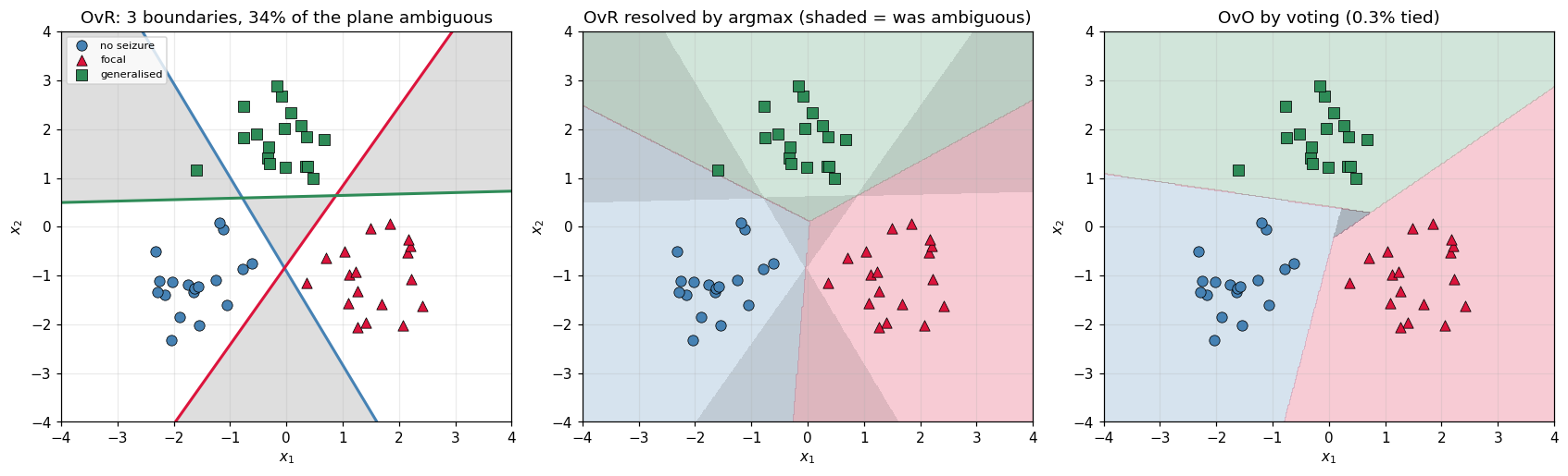
This is not a rare edge case. The cell below sweeps a grid over the whole input region and counts how much of it is undecided. Roughly a third of the plane is ambiguous — including territory sitting right between the training clusters.
==============================================================================
  HOW MUCH OF THE PLANE IS UNDECIDED?
==============================================================================
  grid: 400x400 = 160,000 points over the data region

     machines claiming the point   share of the plane
  ----------------------------------------------------
      none  -> refuses to answer                1.9%
            one   -> unambiguous               65.9%
              two   -> contested               32.3%
              three -> contested                0.0%
  ----------------------------------------------------
     AMBIGUOUS (not exactly one)               34.1%

A point nobody wants
==============================================================================
  x = [-0.251  0.19 ]
              no seizure vs rest: f =  -0.4785  -> not mine
                   focal vs rest: f =  -1.3911  -> not mine
             generalised vs rest: f =  -0.6918  -> not mine
  all three negative. The sign rule returns nothing at all.
  argmax would answer 'no seizure' -- the least unwanted,
  which is a different question from the one we asked.

A point several machines want
==============================================================================
  x = [-3.479  1.414]
              no seizure vs rest: f =   3.3738  -> MINE
                   focal vs rest: f =  -7.8600  -> not mine
             generalised vs rest: f =   1.5055  -> MINE
  2 machines claim it. The sign rule returns a contradiction.

The usual patch: argmax of the raw value instead of the sign
==============================================================================
  Taking argmax_k f_k(x) always returns exactly one class, so the map is
  total. But re-read the ||w|| table above: the three f_k live on
  different scales, so 'most confident' is comparing quantities that
  were never calibrated against each other.

  It works well in practice and it is what scikit-learn's OvR does.
  It is a defensible convention, not a derivation.

Check: does our hand-built OvR match sklearn's?
==============================================================================
  hand-built argmax vs OneVsRestClassifier: 54/54 agree
  training accuracy: ours 1.0000,  sklearn 1.0000
13.2 One-vs-One: every pair votes
The alternative avoids the "rest" entirely. Train one machine for each pair of classes, using only the data from those two:
$$\binom{K}{2} = \frac{K(K-1)/1}{2} \quad\text{machines} \qquad K=3 \;\Rightarrow\; 3 \quad\text{but} \quad K=10 \;\Rightarrow\; 45$$
Each machine votes for one of its two classes; the class with most votes wins.
Two things make this attractive despite the larger number of machines:
- each problem is smaller. With $K$ balanced classes, a pair-machine sees about $2n/K$ points instead of all $n$. Kernel SVM training scales worse than linearly in $n$, so many small problems can be cheaper than a few large ones.
- each problem is balanced. OvR's "rest" class is $K-1$ times larger than the "one", which is exactly the imbalance the [[evaluation-metrics]] page warns about.
The cost is that voting can tie, and unlike OvR's ambiguity a tie has no natural ordering to fall back on.
==============================================================================
  ONE-VS-ONE: PAIRWISE MACHINES AND A VOTE
==============================================================================
  K = 3  ->  K(K-1)/2 = 3 machines

                          pair   n used    of     ||w||
  ------------------------------------------------------
           no seizure vs focal       36    54    1.4291
     no seizure vs generalised       36    54    1.5396
          focal vs generalised       36    54    1.4075
  ------------------------------------------------------
  each machine used 36 of 54 epochs (67%), and its two classes are balanced

The vote for one epoch, written out
==============================================================================
  epoch at [-0.6163 -0.7599], true class = no seizure

                       machine       f(x)  votes for
  --------------------------------------------------------
           no seizure vs focal     0.8042  no seizure
     no seizure vs generalised     1.9353  no seizure
          focal vs generalised    -0.0273  generalised
  --------------------------------------------------------
                         tally
                    no seizure  2 vote(s)  ##
                         focal  0 vote(s)
                   generalised  1 vote(s)  #

  winner: no seizure   (true: no seizure)
  unique winner: True

Ties are possible, and they have no natural resolution
==============================================================================
  With K=3 a 1-1-1 tie happens when the three machines disagree in a
  cycle: A beats B, B beats C, C beats A. Nothing about the votes
  themselves breaks it.
  over the same 160,000-point grid, ties occur on 0.25% of the plane
  compare one-vs-rest's 34.1% ambiguous area

  sklearn breaks remaining ties with the summed decision values, so the
  predictor is total either way -- but OvO has far less to patch over.

Check: does our hand-built OvO match sklearn's SVC?
==============================================================================
  SVC decision_function shape = (54, 3)  -> 3 columns, one per PAIR: SVC is one-vs-one
  hand-built vote vs SVC.predict: 54/54 agree
  training accuracy: ours 1.0000,  sklearn 1.0000
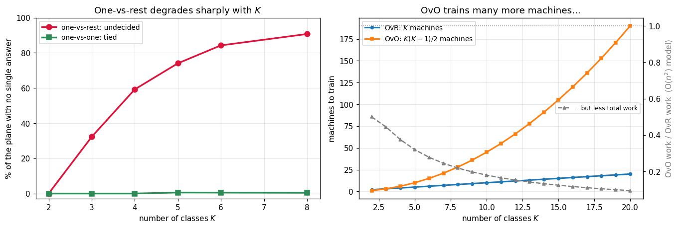
13.3 Any number of classes, and why $K$ matters more than it looks
Three classes was only an example. Both schemes are defined for any $K$, and the formulas above are already general:
$$\text{OvR: } K \text{ machines} \qquad\qquad \text{OvO: } \binom{K}{2} = \frac{K(K-1)}{2} \text{ machines}$$
What is not obvious from the formulas is that the two schemes degrade very differently as $K$ grows. The count of machines is the visible difference — OvO grows quadratically and looks worse. The invisible difference matters more.
For each machine in one-vs-rest, the positive class is one class and the negative class is the other $K-1$ combined. At $K=10$ that is a 1:9 imbalance in every single machine, and the boundary is pushed toward the small class. Worse, each machine is drawing a boundary in a space where $K-1$ distinct clusters sit on the negative side — a single hyperplane is a poor summary of "everything that is not class $k$".
The sweep below repeats the ambiguity measurement for $K = 2 \dots 8$. The result is stronger than the $K=3$ figure suggested.
==============================================================================
  HOW THE TWO SCHEMES SCALE WITH THE NUMBER OF CLASSES
==============================================================================
  18 epochs per class, classes placed evenly on a circle
  ambiguity measured over a 260x260 grid

    K    OvR    OvO   pts/OvR   pts/OvO   OvR ambiguous   OvO tied
  --------------------------------------------------------------------
    2      2      1        36        36           0.0%      0.0%
    3      3      3        54        36          32.3%      0.0%
    4      4      6        72        36          59.3%      0.0%
    5      5     10        90        36          74.1%      0.6%
    6      6     15       108        36          84.3%      0.5%
    8      8     28       144        36          90.7%      0.4%
  --------------------------------------------------------------------

The column that matters
==============================================================================
  One-vs-rest ambiguity, as K grows:
    K = 2:   0.0%
    K = 3:  32.3%  ###############
    K = 4:  59.3%  ###########################
    K = 5:  74.1%  #################################
    K = 6:  84.3%  ######################################
    K = 8:  90.7%  #########################################

  At K = 2 there is nothing to be ambiguous about -- one machine, two
  sides, 0% undecided. By K = 8 the sign rule fails to give a
  single answer on 91% of the plane.

  One-vs-one over the same range:
    K = 2:   0.0%
    K = 3:   0.0%
    K = 4:   0.0%
    K = 5:   0.6%
    K = 6:   0.5%
    K = 8:   0.4%
  Ties stay under 1% throughout.

Why one-vs-rest degrades this way
==============================================================================
     K   positive   negative   imbalance
  ----------------------------------------
     2         18         18  1 : 1
     3         18         36  1 : 2
     5         18         72  1 : 4
    10         18        162  1 : 9
    20         18        342  1 : 19
  ----------------------------------------
  Every OvR machine is a 1-against-many problem, and 'many' is not one
  blob -- it is K-1 separate clusters. Asking a single hyperplane to
  wrap around all of them is asking the wrong question, and the
  undecided regions are where it fails to answer.

  One-vs-one never poses that question. Every machine it trains is a
  balanced, two-cluster problem of exactly the kind the rest of this
  page is about.

Cost, for a kernel SVM
==============================================================================
  Kernel SVM training is roughly O(n^2) to O(n^3). Take O(n^2) and
  n = 18 points per class:

     K    OvR total work    OvO total work     ratio
  --------------------------------------------------
     2             2,592             1,296      0.50x
     3             8,748             3,888      0.44x
     5            40,500            12,960      0.32x
    10           324,000            58,320      0.18x
    20         2,592,000           246,240      0.10x
  --------------------------------------------------
  OvO trains far more machines and still does less total work, because
  each one sees a fixed 2n/K slice while every OvR machine sees all n.
  This is why libsvm -- and therefore SVC -- picked one-vs-one.
13.4 Which to use
| One-vs-Rest | One-vs-One | |
|---|---|---|
| machines for $K$ classes | $K$ | $K(K-1)/2$ |
| $K=3$ | 3 | 3 |
| $K=10$ | 10 | 45 |
| points per machine | all $n$ | $\approx 2n/K$ |
| class balance | 1 : $(K-1)$ — skewed | 1 : 1 |
| failure mode | undecided regions | tied votes |
| scikit-learn | LinearSVC, OneVsRestClassifier |
SVC (default) |
SVC uses one-vs-one, which is why its decision_function returns
$K(K-1)/2$ columns rather than $K$ — a detail that surprises people reading
those numbers as per-class scores.
The number of machines makes OvR look cheaper, and for a linear model it usually
is. For a kernel SVM it often is not: training cost grows faster than linearly in
$n$, so 45 machines on $n/5$ points each can beat 10 machines on all $n$. That
tradeoff is the actual reason libsvm — and therefore SVC — chose OvO.
What to carry forward
- An SVM is binary. Multi-class is an ensemble, and the combination rule is a design choice, not something the optimisation hands you.
- One-vs-rest leaves the space undecided. Measured here at 34% of the plane: 2% claimed by nobody, 32% contested. The
argmaxpatch makes the predictor total, but it compares decision values from machines with different $\lVert\mathbf{w}\rVert$ — a convention rather than a result. - One-vs-one trades more machines for smaller, balanced ones, and ties over far less of the space.
- Neither scheme maximises a single margin over all classes. Formulations that do exist (Crammer–Singer,
LinearSVC(multi_class="crammer_singer")), solving one joint problem instead of composing binary ones — they are less used, mostly because the decomposition approaches work well enough and parallelise trivially.
14. Summary
| Concept | Formula |
|---|---|
| Margin | $2/\lVert\mathbf{w}\rVert$ |
| Primal | $\tfrac12\lVert\mathbf{w}\rVert^2 + C\sum_i\max(0, 1-y_i f(\mathbf{x}_i))$ |
| Dual | $\sum_i\alpha_i - \tfrac12\sum_{i,j}\alpha_i\alpha_j y_iy_j K(\mathbf{x}_i,\mathbf{x}_j)$ |
| Recover $\mathbf{w}$ | $\sum_i \alpha_i y_i \mathbf{x}_i$ |
| Predict | $\operatorname{sign}\big(\sum_{i\in SV}\alpha_i y_i K(\mathbf{x}_i,\mathbf{x}) + b\big)$ |
| Support vector | $\alpha_i > 0$, i.e. on or inside the margin |
| $C$ | large = narrow margin, few violations |
| $\gamma$ (RBF) | large = tight, local bubbles = overfitting |
The one idea: write the problem so the data appears only as inner products, and every inner product becomes a free choice. That is the kernel trick, and it turns a linear classifier into a family that includes infinite-dimensional feature spaces.
The practical cost: the dual is $O(n^2)$ to $O(n^3)$ in the number of samples, and the kernel matrix is $n \times n$. SVMs are excellent up to tens of thousands of rows and impractical at millions — which is precisely the range where the gradient-boosted trees in this series take over.
What is deliberately left out: the KKT conditions and how $b$ is recovered from them, the SMO algorithm that actually solves the dual, multi-class strategies (one-vs-one, one-vs-rest), probability calibration via Platt scaling, and the $\nu$-SVM parameterisation.