📏 Support Vector Regression
Support vector regression takes the SVM machinery — margins, support vectors, kernels — and points it at a continuous target. The translation rests on one inversion:
Classification: keep points outside the margin. Regression: keep points inside a tube.
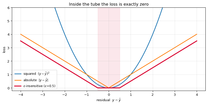
Least squares penalises every residual, however small. SVR ignores errors below a tolerance $\varepsilon$ entirely:
$$L_\varepsilon(y, \hat y) = \max\big(0,\; |y - \hat y| - \varepsilon\big)$$
That flat region has real consequences. Points inside the tube have zero gradient, so they contribute nothing and are discarded — giving a sparse model built from a few boundary points, just like the classifier. And because errors below $\varepsilon$ cost nothing, the fit is insensitive to small noise while remaining only linearly — not quadratically — sensitive to outliers.
Display helpers ready: banner, step, check, expand, show_matrix, show_matmul, show_elementwise.
1. The Data
The 12 EEG recordings with the continuous target y_reg (seizure burden, minutes/hour),
the same one used in the XGBoost walkthrough.
Features are standardised: SVR measures distances in feature space, so unscaled columns would dominate the kernel exactly as they do for KNN and SVM.
12 recordings x 3 features

    id      region   line_length    spike_rate           age   y_class    y_reg
-------------------------------------------------------------------------------
 rec00     frontal          12.0           0.5          24.0         0      0.2
 rec01    temporal          15.0           1.2          31.0         0      0.5
 rec02    temporal          42.0           6.8          58.0         1      6.4
 rec03   occipital          38.0           5.1          47.0         1      4.8
 rec04     frontal          11.0           0.3          19.0         0      0.1
 rec05    temporal          55.0           8.2          63.0         1      9.1
 rec06   occipital          40.0           1.9          35.0         1      3.5
 rec07    temporal          47.0           7.4          52.0         1      7.2
 rec08     frontal          14.0           0.8          28.0         0      0.3
 rec09   occipital          51.0           6.1          60.0         1      6.9
 rec10     frontal          45.0           2.4          41.0         0      1.6
 rec11    temporal          35.0           4.7          30.0         1      4.1
-------------------------------------------------------------------------------

class balance: 5 negative, 7 positive
y_reg mean = 3.7250, std = 3.0518
target y: mean 3.7250, std 3.0518, range [0.1, 9.1]

standardised features:

X (standardised) (12, 3) =
             line_lengthspike_rate       age
        rec00 |   -1.397    -1.176    -1.157
        rec01 |   -1.204    -0.925    -0.671
        rec02 |   +0.530    +1.080    +1.204
        rec03 |   +0.273    +0.472    +0.440
        rec04 |   -1.461    -1.247    -1.505
        rec05 |   +1.365    +1.582    +1.551
        rec06 |   +0.401    -0.674    -0.393
        rec07 |   +0.851    +1.295    +0.787
        rec08 |   -1.268    -1.068    -0.880
        rec09 |   +1.108    +0.830    +1.342
        rec10 |   +0.722    -0.495    +0.023
        rec11 |   +0.080    +0.328    -0.741
2. The $\varepsilon$-Insensitive Tube
$$\min_{\mathbf{w},b,\xi,\xi^*} \;\; \frac{1}{2}\lVert\mathbf{w}\rVert^2 + C\sum_i(\xi_i + \xi_i^*)$$
$$\text{s.t.}\quad \begin{cases} y_i - (\mathbf{w}^\top\mathbf{x}_i + b) \le \varepsilon + \xi_i \\[2pt] (\mathbf{w}^\top\mathbf{x}_i + b) - y_i \le \varepsilon + \xi_i^* \\[2pt] \xi_i, \xi_i^* \ge 0 \end{cases}$$
Two slack variables are needed because a point can miss the tube from above or below, and those are different violations.
Compare the three loss shapes:
| Loss | Formula | Behaviour |
|---|---|---|
| Squared | $(y-\hat y)^2$ | every error counts; outliers dominate |
| Absolute | $\lvert y-\hat y\rvert$ | robust, but every error still counts |
| $\varepsilon$-insensitive | $\max(0, \lvert y-\hat y\rvert - \varepsilon)$ | small errors are free |
residual    squared   absolute   eps-insensitive
--------------------------------------------------
       0.0      0.000      0.000             0.000
       0.2      0.040      0.200             0.000
       0.5      0.250      0.500             0.000
       1.0      1.000      1.000             0.500
       2.0      4.000      2.000             1.500
       4.0     16.000      4.000             3.500
--------------------------------------------------

At a residual of 0.2 the squared loss still pushes back; the
eps-insensitive loss is flat, so that point exerts NO force on the fit.
At a residual of 4 the squared loss is 4.6x larger - which is
why least squares is dragged around by outliers and SVR is not.
3. The Tube on Real Data
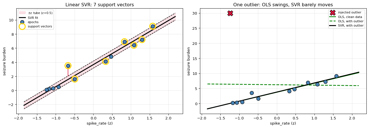
Fitting a linear SVR to one feature makes the geometry visible: a central line, two dashed walls at $\pm\varepsilon$, and support vectors circled.
linear SVR on 'spike_rate' alone   (C = 10.0, epsilon = 0.5)

   w = +3.127600   b = +3.649334
   support vectors: 7 of 12

    id     x (z)        y      pred   residual    |r|-eps            status
------------------------------------------------------------------------
 rec06   -0.6744     3.50    1.5400     1.9600     1.4600    SUPPORT VECTOR
 rec09    0.8296     6.90    6.2440     0.6560     0.1560    SUPPORT VECTOR
 rec02    1.0803     6.40    7.0280    -0.6280     0.1280    SUPPORT VECTOR
 rec11    0.3283     4.10    4.6760    -0.5760     0.0760    SUPPORT VECTOR
 rec05    1.5816     9.10    8.5960     0.5040     0.0040    SUPPORT VECTOR
 rec07    1.2951     7.20    7.7000    -0.5000     0.0000    SUPPORT VECTOR
 rec10   -0.4954     1.60    2.1000    -0.5000     0.0000    SUPPORT VECTOR
 rec04   -1.2474     0.10   -0.2520     0.3520    -0.1480       inside tube
 rec03    0.4715     4.80    5.1240    -0.3240    -0.1760       inside tube
 rec01   -0.9251     0.50    0.7560    -0.2560    -0.2440       inside tube
 rec00   -1.1758     0.20   -0.0280     0.2280    -0.2720       inside tube
 rec08   -1.0683     0.30    0.3080    -0.0080    -0.4920       inside tube
------------------------------------------------------------------------

points strictly inside the tube : 5
points on or outside the tube   : 7
sklearn's support vectors        : 7

The two counts agree here: a point is a support vector when it is NOT
strictly inside the tube, and everything inside could be deleted.

That rule is exact in principle; section 6 shows the one place it gets
blurry, where a point sits on the tube wall to within solver tolerance.
slope with clean data      : OLS +2.9724   SVR +3.1276
slope after one outlier    : OLS -0.1357   SVR +3.0177
change                     : OLS +3.1081   SVR +0.1099

OLS moved 28.3x more than SVR. The squared loss grows without bound; the
eps-insensitive loss grows only linearly, so one bad point cannot dominate.
4. What $\varepsilon$ and $C$ Do
They pull in different directions:
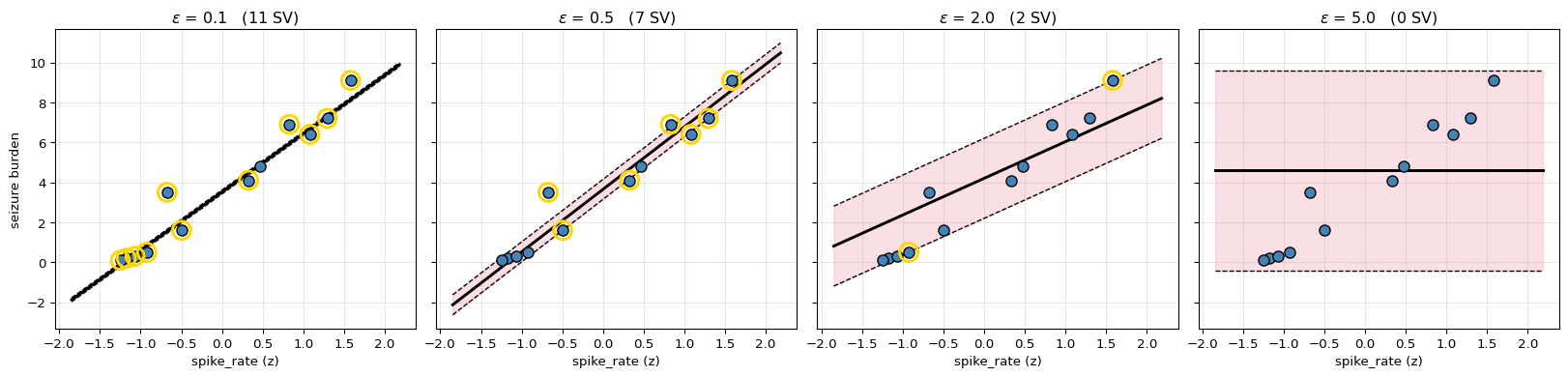
- $\varepsilon$ sets the tube width. Wider tube → more points inside → fewer support vectors → a simpler, flatter model. At $\varepsilon$ larger than the spread of $y$, every point fits inside and the model collapses to a constant.
- $C$ sets the price of leaving the tube. Large $C$ → violations are expensive → the fit bends to accommodate them.
epsilon    #SV      ||w||    train MSE   mean |resid|
--------------------------------------------------------
     0.00     12     2.1562       0.6527         0.3962
     0.25      7     2.1527       0.4244         0.4314
     0.50      5     2.2364       0.4535         0.4873
     1.00      5     2.6147       0.7047         0.7761
     2.00      2     1.3172       1.4003         1.0150
     4.00      2     0.1987       8.2204         2.4906
     8.00      0     0.0000      10.0792         2.7750
--------------------------------------------------------

(the spread of y is 9.0, so epsilon = 8 swallows nearly
 everything and the model gives up)

        C    #SV      ||w||    train MSE
----------------------------------------
     0.01     10     0.1644       7.7968
     0.10     10     1.3176       1.2068
     1.00      5     1.8339       0.5774
    10.00      5     2.2364       0.4535
   100.00      6     2.8242       0.4168
  1000.00      6     2.8240       0.4167
----------------------------------------

Small C keeps ||w|| tiny and underfits badly; large C chases the data.
As the tube widens the gold circles disappear one by one - the model is
built from fewer and fewer points, and eventually stops tracking the data.
5. Kernels, and Prediction Through Them
The dual has the same shape as the classifier's, and again the data enters only through inner products. So the same kernels apply, and prediction is:
$$f(\mathbf{x}) = \sum_{i \in SV}(\alpha_i - \alpha_i^{*})\,K(\mathbf{x}_i, \mathbf{x}) + b$$
sklearn stores the combined coefficient $(\alpha_i - \alpha_i^{*})$ in dual_coef_.
Below that sum is evaluated by hand and checked against predict.
predicting rec05 (true y = 9.10)

     SV   alpha-alpha*     K(sv,x)      product
----------------------------------------------
  rec01       -2.10722    0.000135    -0.000285
  rec03        1.46736    0.160542     0.235572
  rec04       -2.22656    0.000003    -0.000007
  rec05        4.59669    1.000000     4.596690
  rec06        4.95842    0.007455     0.036964
  rec10       -6.68870    0.029305    -0.196011
----------------------------------------------
    sum                                4.672923

f(x) = 4.672923 + b(+3.927051) = 8.599974
sklearn predict            = 8.599974
MATCH: True

all 12 predictions by hand MATCH sklearn: True


coefficients are bounded by C = 10.0:
   max |alpha - alpha*| = 6.688696
   all within [-C, C]? True
   at the bound (fully outside the tube): 0 of 6
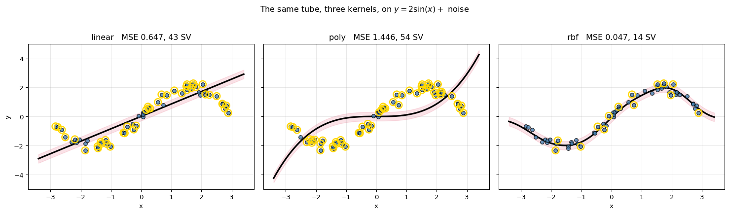
kernel        MSE    #SV   SV fraction
------------------------------------------
    linear     0.6474     43        71.7%
      poly     1.4457     54        90.0%
       rbf     0.0470     14        23.3%
------------------------------------------

The RBF fit tracks the sine closely while still ignoring every point that
lands inside the tube - accuracy and sparsity at the same time.
6. Checking Against scikit-learn
linear SVR: recover w from the dual coefficients
----------------------------------------------------------
w = sum_i (alpha_i - alpha_i*) x_i
   from dual   : [0.7688 2.0932 0.1698]
   sklearn coef: [0.7688 2.0932 0.1698]
   MATCH: True

predictions by hand MATCH sklearn: True


the eps-insensitive loss, evaluated directly
----------------------------------------------------------
   0.5*||w||^2       = 2.500772
   C * sum of losses = 10.0 * 1.593203 = 15.932028
   objective         = 18.432799
   random perturbations that beat it: 0/4000


the support-vector rule, and where solver tolerance shows up
----------------------------------------------------------
     id    |resid| - eps            region    SV?   alpha-alpha*
----------------------------------------------------------------
  rec00        -4.55e-01            inside     no              0
  rec09        -3.93e-01            inside     no              0
  rec04        -3.87e-01            inside     no              0
  rec07        -2.25e-01            inside     no              0
  rec08        -1.84e-01            inside     no              0
  rec03        -5.19e-02            inside     no              0
  rec02        -5.05e-02            inside     no              0
  rec11        -2.74e-04   ON the boundary    yes       -0.75684
  rec05         2.75e-04   ON the boundary    yes       +1.92775
  rec01         5.49e-04   ON the boundary    yes       -1.17091
  rec06         1.93e-01           outside    yes      +10.00000
  rec10         1.40e+00           outside    yes      -10.00000
----------------------------------------------------------------

   clearly inside  (7): any of them support vectors? False
   clearly outside (2): all of them support vectors? True
   on the boundary (3): decided by the solver, not by us

   In exact arithmetic a point is a support vector precisely when it is
   not strictly inside the tube. libsvm stops at tol = 0.001, so points
   sitting within that distance of the wall can be kept with a small
   non-zero alpha - see the boundary rows above, whose |alpha| are the
   smallest in the model while the far-outside points sit at C = 10.0.
7. Summary
| Concept | Formula |
|---|---|
| Loss | $\max(0, \lvert y-\hat y\rvert - \varepsilon)$ |
| Objective | $\tfrac12\lVert\mathbf{w}\rVert^2 + C\sum_i(\xi_i+\xi_i^{*})$ |
| Predict | $\sum_{i\in SV}(\alpha_i-\alpha_i^{*})K(\mathbf{x}_i,\mathbf{x}) + b$ |
| Support vector | any point not strictly inside the tube |
| $\varepsilon$ larger | wider tube, fewer SVs, simpler model |
| $C$ larger | violations costlier, fit bends more |
The one idea: make the loss flat near zero. That single change turns a regression into a sparse, margin-based problem — the points that fit well drop out of the model entirely, and the ones that remain define it.
Why it resists outliers: beyond $\varepsilon$ the penalty grows linearly, not quadratically. A point ten units away is ten times as costly, not a hundred times, so it cannot dominate the fit the way it does in least squares.
What is deliberately left out: the full dual derivation with both $\alpha$ and $\alpha^{*}$, the KKT conditions, $\nu$-SVR (which sets the fraction of support vectors instead of $\varepsilon$), and the $O(n^2)$–$O(n^3)$ scaling that makes SVR impractical on large datasets.