⚡ XGBoost
A random forest grows its trees independently and averages them. Boosting does the opposite: trees are grown one at a time, and every new tree is fitted to the part of the answer the previous trees got wrong.
XGBoost's contribution is to make that idea exact. Instead of fitting the residuals heuristically, it writes down the loss, takes a second-order Taylor expansion, and derives — in closed form — both the best value for a leaf and the gain of a split.
Two quantities do all the work:
$$g_i = \frac{\partial\, l(y_i, \hat y_i)}{\partial \hat y_i} \qquad\qquad h_i = \frac{\partial^2 l(y_i, \hat y_i)}{\partial \hat y_i^2}$$
Everything below — leaf weights, split gains, pruning — is built from sums of these
two numbers. At the end every split and every leaf value is compared against the real
xgboost library, and they agree to the last decimal.
Display helpers ready: banner, step, check, expand, show_matrix, show_matmul, show_elementwise.
Tree diagram helper ready: draw_tree(root, title).
1. The Task
Same 12 EEG recordings, but now a regression target: y_reg, the seizure burden in
minutes per hour. Boosting is easiest to follow on squared error, where the derivatives
are as simple as they get.
12 recordings x 3 features

    id      region   line_length    spike_rate           age   y_class    y_reg
-------------------------------------------------------------------------------
 rec00     frontal          12.0           0.5          24.0         0      0.2
 rec01    temporal          15.0           1.2          31.0         0      0.5
 rec02    temporal          42.0           6.8          58.0         1      6.4
 rec03   occipital          38.0           5.1          47.0         1      4.8
 rec04     frontal          11.0           0.3          19.0         0      0.1
 rec05    temporal          55.0           8.2          63.0         1      9.1
 rec06   occipital          40.0           1.9          35.0         1      3.5
 rec07    temporal          47.0           7.4          52.0         1      7.2
 rec08     frontal          14.0           0.8          28.0         0      0.3
 rec09   occipital          51.0           6.1          60.0         1      6.9
 rec10     frontal          45.0           2.4          41.0         0      1.6
 rec11    temporal          35.0           4.7          30.0         1      4.1
-------------------------------------------------------------------------------

class balance: 5 negative, 7 positive
y_reg mean = 3.7250, std = 3.0518
objective   : reg:squarederror,  l(y, p) = 0.5 * (y - p)^2
base_score  : 0.5
eta         : 0.3
lambda (L2) : 1.0
gamma       : 0.0
max_depth   : 2

target y = [0.2 0.5 6.4 4.8 0.1 9.1 3.5 7.2 0.3 6.9 1.6 4.1]
mean(y) = 3.7250
2. Gradients and Hessians
XGBoost minimises
$$\mathcal{L} = \sum_i l(y_i, \hat y_i) \;+\; \sum_k \Omega(f_k), \qquad \Omega(f) = \gamma T + \tfrac{1}{2}\lambda \sum_{j=1}^{T} w_j^2$$
where $T$ is the number of leaves and $w_j$ their values. Adding a new tree $f_t$ to the current prediction and expanding the loss to second order:
$$\mathcal{L}^{(t)} \simeq \sum_i \Big[\, g_i f_t(x_i) + \tfrac{1}{2} h_i f_t(x_i)^2 \Big] + \Omega(f_t) + \text{const}$$
The whole training set is now summarised by two numbers per row. The original $y$ never appears again — only $g$ and $h$.
For squared error $l(y,\hat y) = \tfrac12 (y - \hat y)^2$:
$$g_i = \hat y_i - y_i \qquad\qquad h_i = 1$$
so the gradient is simply the negative residual, and every Hessian is 1.
round 1: every prediction starts at base_score = 0.5

    id        y     pred   residual (y-p)    g = p - y     h
------------------------------------------------------------
 rec00     0.20     0.50            -0.30         0.30     1
 rec01     0.50     0.50             0.00         0.00     1
 rec02     6.40     0.50             5.90        -5.90     1
 rec03     4.80     0.50             4.30        -4.30     1
 rec04     0.10     0.50            -0.40         0.40     1
 rec05     9.10     0.50             8.60        -8.60     1
 rec06     3.50     0.50             3.00        -3.00     1
 rec07     7.20     0.50             6.70        -6.70     1
 rec08     0.30     0.50            -0.20         0.20     1
 rec09     6.90     0.50             6.40        -6.40     1
 rec10     1.60     0.50             1.10        -1.10     1
 rec11     4.10     0.50             3.60        -3.60     1
------------------------------------------------------------
   SUM    44.70     6.00            38.70       -38.70    12

G = sum of g = -38.7000      H = sum of h = 12

A large negative G means the model is under-predicting overall,
which it is: every prediction is 0.5 but mean(y) = 3.725.
3. The Optimal Leaf Weight
Take a single leaf holding a set of rows $I$. Every row in it receives the same output $w$, so the objective restricted to that leaf is a plain quadratic in $w$:
$$\mathcal{L}_{\text{leaf}}(w) = \Big(\sum_{i \in I} g_i\Big) w + \tfrac{1}{2}\Big(\sum_{i \in I} h_i + \lambda\Big) w^2 = G w + \tfrac{1}{2}(H + \lambda) w^2$$
Differentiate, set to zero, and the best possible value of that leaf falls out:
$$\frac{d\mathcal{L}}{dw} = G + (H+\lambda)w = 0 \qquad\Longrightarrow\qquad \boxed{\;w^{*} = -\frac{G}{H + \lambda}\;}$$
Substituting $w^*$ back gives the best achievable objective for that leaf:
$$\mathcal{L}^{*}_{\text{leaf}} = -\frac{1}{2}\,\frac{G^2}{H+\lambda}$$
The quantity $\dfrac{G^2}{H+\lambda}$ is called the similarity score (or structure score). A leaf is good when its rows agree — their gradients point the same way and add up instead of cancelling.
If the whole dataset were ONE leaf:

   G = (+0.30) + (+0.00) + (-5.90) + (-4.30) + (+0.40) + (-8.60) + ...
     = -38.700000
   H = 12  (one per row, since h_i = 1)

   w* = -G / (H + lambda) = -(-38.7000) / (12 + 1.0)
      = 38.7000 / 13.0 = +2.976923

   similarity = G^2 / (H + lambda) = (-38.7000)^2 / 13.0
              = 1497.6900 / 13.0 = 115.206923

Sanity: the unregularised optimum would be the mean residual,
   -G/H = +3.225000   vs   mean(y - pred) = +3.225000   MATCH: True

lambda = 1.0 shrinks it from +3.225000 to +2.976923 -
that shrinkage IS the L2 regularisation.
What $\lambda$ does to a leaf
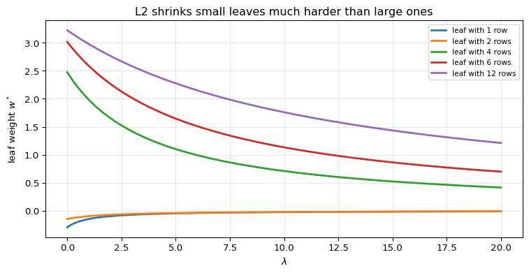
$\lambda$ pulls every leaf weight toward zero, and it bites hardest on small leaves: a leaf with 6 rows has $H = 6$, so $\lambda = 1$ changes it by about 14%, while a leaf with one row has $H = 1$ and is halved.
That is deliberate. Leaves supported by little evidence should not be trusted.
leaf size         G     H  lam=0      lam=1      lam=5      lam=20
------------------------------------------------------------
         1      0.30     1  -0.3000    -0.1500    -0.0500    -0.0143
         2      0.30     2  -0.1500    -0.1000    -0.0429    -0.0136
         4     -9.90     4  2.4750     1.9800     1.1000     0.4125
         6    -18.10     6  3.0167     2.5857     1.6455     0.6962
        12    -38.70    12  3.2250     2.9769     2.2765     1.2094
------------------------------------------------------------
Small leaves collapse toward zero quickly; the 12-row leaf barely moves.
4. The Gain of a Split
Splitting a node replaces one leaf by two. The improvement is the similarity the two children have together minus what the parent had alone, minus the cost $\gamma$ of adding a leaf:
$$\text{Gain} = \frac{1}{2}\left[ \frac{G_L^2}{H_L+\lambda} + \frac{G_R^2}{H_R+\lambda} - \frac{(G_L+G_R)^2}{H_L+H_R+\lambda} \right] - \gamma$$
A split helps when it puts rows with similar gradients together, so that they reinforce instead of cancelling.
A detail worth knowing: the
xgboostmodel dump reports this quantity without the $\tfrac{1}{2}$ — exactly twice the value above. The factor is constant, so it never changes which split wins, but the printed numbers differ by 2x. Both are shown below.
All 33 candidate splits for TREE 0, ranked

rank       feature       thr   nL       G_L   nR       G_R   gain (xgb)       GAIN
----------------------------------------------------------------------------------
   1    spike_rate      3.55    6     -3.20    6    -35.50      66.2916    33.1458  <== BEST
   2    spike_rate      4.90    7     -6.80    5    -31.90      60.1747    30.0874
   3           age     44.00    7     -6.80    5    -31.90      60.1747    30.0874
   4   line_length     25.00    4      0.90    8    -39.60      59.1951    29.5975
   5    spike_rate      1.55    4      0.90    8    -39.60      59.1951    29.5975
   6    spike_rate      2.15    5     -2.10    7    -36.60      52.9731    26.4865
   7    spike_rate      5.60    8    -11.10    4    -27.60      50.8351    25.4175
   8           age     49.50    8    -11.10    4    -27.60      50.8351    25.4175
   9   line_length     36.50    5     -2.70    7    -36.00      48.0081    24.0040
  10           age     33.00    5     -2.70    7    -36.00      48.0081    24.0040
  11           age     38.00    6     -5.70    6    -33.00      45.0059    22.5030
  12   line_length     14.50    3      0.90    9    -39.60      41.8116    20.9058
  13    spike_rate      1.00    3      0.90    9    -39.60      41.8116    20.9058
  14           age     29.00    3      0.90    9    -39.60      41.8116    20.9058
  15   line_length     39.00    6     -7.00    6    -31.70      35.3488    17.6744
  16   line_length     41.00    7    -10.00    5    -28.70      34.5747    17.2874
  17   line_length     46.00    9    -17.00    3    -21.70      31.4156    15.7078
  18           age     30.50    4     -2.70    8    -36.00      30.2511    15.1255
  19    spike_rate      6.45    9    -17.50    3    -21.20      27.7781    13.8890
  20   line_length     13.00    2      0.70   10    -39.40      26.0800    13.0400
  21    spike_rate      0.65    2      0.70   10    -39.40      26.0800    13.0400
  22           age     26.00    2      0.70   10    -39.40      26.0800    13.0400
  23           age     55.00    9    -17.80    3    -20.90      25.6796    12.8398
  24   line_length     43.50    8    -15.90    4    -22.80      16.8511     8.4255
  25    spike_rate      7.10   10    -23.40    2    -15.30      12.6013     6.3006
  26   line_length     11.50    1      0.40   11    -39.10      12.2739     6.1370
  27    spike_rate      0.40    1      0.40   11    -39.10      12.2739     6.1370
  28           age     21.50    1      0.40   11    -39.10      12.2739     6.1370
  29   line_length     49.00   10    -23.70    2    -15.00      10.8558     5.4279
  30           age     59.00   10    -23.70    2    -15.00      10.8558     5.4279
  31   line_length     53.00   11    -30.10    1     -8.60      -2.7261    -1.3630
  32    spike_rate      7.80   11    -30.10    1     -8.60      -2.7261    -1.3630
  33           age     61.50   11    -30.10    1     -8.60      -2.7261    -1.3630
----------------------------------------------------------------------------------

WINNER: spike_rate <= 3.55

   LEFT  (6 rows): G_L = -3.2000, H_L = 6  ->  S_L = (-3.2000)^2 / 7.0 = 1.4629
   RIGHT (6 rows): G_R = -35.5000, H_R = 6  ->  S_R = (-35.5000)^2 / 7.0 = 180.0357
   PARENT: S_P = 115.2069

   Gain = 0.5 * [ 1.4629 + 180.0357 - 115.2069 ] - 0.0
        = 0.5 * 66.2916 = 33.145824
   xgboost will report this as 66.291648 (no 1/2 factor)
5. Growing Tree 0
The split search recurses exactly like a decision tree, but the score is the gain above
rather than Gini. At max_depth = 2 the tree stops and every remaining node becomes a
leaf with weight $w^* = -G/(H+\lambda)$.
Finally each leaf is multiplied by the learning rate $\eta$. Shrinkage means no single tree is trusted completely — it takes a small step and leaves the rest for later trees.
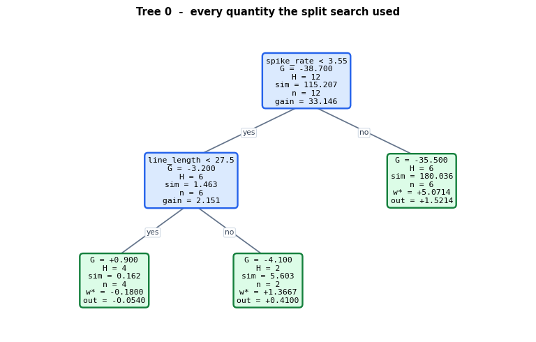
TREE 0, built from the formulas alone:

[spike_rate < 3.55]  gain=66.2916 (xgb) / 33.1458 (with 1/2)  cover=12
|-- yes: [line_length < 27.5]  gain=4.3025 (xgb) / 2.1512 (with 1/2)  cover=6
    |-- yes: LEAF  raw w* = -0.180000   x eta = -0.054000   cover=4  rows=['00', '01', '04', '08']
    |-- no : LEAF  raw w* = +1.366667   x eta = +0.410000   cover=2  rows=['06', '10']
|-- no : LEAF  raw w* = +5.071429   x eta = +1.521429   cover=6  rows=['02', '03', '05', '07', '09', '11']
Reading a node:
   G, H   sums of the gradients and Hessians of the rows reaching it
   sim    similarity G^2/(H+lambda) - how much the rows agree
   gain   0.5 * [sim_L + sim_R - sim_parent] - gamma
   w*     the closed-form optimal leaf value, -G/(H+lambda)
   out    what the tree actually adds: eta * w*

leaf arithmetic, one by one:

leaf 0: rows ['00', '01', '04', '08']
   G = (+0.30) + (+0.00) + (+0.40) + (+0.20) = +0.9000
   H = 4,  w* = -(+0.9000) / (4 + 1.0) = -0.180000
   output after shrinkage = 0.3 * -0.180000 = -0.054000

leaf 1: rows ['06', '10']
   G = (-3.00) + (-1.10) = -4.1000
   H = 2,  w* = -(-4.1000) / (2 + 1.0) = +1.366667
   output after shrinkage = 0.3 * +1.366667 = +0.410000

leaf 2: rows ['02', '03', '05', '07', '09', '11']
   G = (-5.90) + (-4.30) + (-8.60) + (-6.70) + (-6.40) + (-3.60) = -35.5000
   H = 6,  w* = -(-35.5000) / (6 + 1.0) = +5.071429
   output after shrinkage = 0.3 * +5.071429 = +1.521429
6. Checking Tree 0 Against the Real XGBoost
Training xgboost with the identical hyper-parameters and dumping the booster should
reproduce the same split, the same gain, and the same leaf outputs.
xgboost's own dump of tree 0:

0:[spike_rate<3.54999995] yes=1,no=2,missing=1,gain=66.2916565,cover=12
	1:[line_length<27.5] yes=3,no=4,missing=3,gain=4.30247593,cover=6
		3:leaf=-0.0540000051,cover=4
		4:leaf=0.410000026,cover=2
	2:leaf=1.5214287,cover=6

root gain   : ours x2 =     66.29165  |  xgboost =     66.29166  MATCH: True
root feature: ours = spike_rate, threshold 3.55

 leaf    ours (eta * w*)         xgboost        diff
----------------------------------------------------
    0         -0.0540000      -0.0540000    5.10e-09
    1          0.4100000       0.4100000    2.60e-08
    2          1.5214286       1.5214287    1.29e-07
----------------------------------------------------

all leaf outputs MATCH: True
Predictions after one tree
$$\hat y^{(1)}_i = \text{base\_score} + \eta \, w^{*}_{\text{leaf}(i)}$$
id        y    pred0    w* leaf    eta*w*     pred1    xgboost       diff
-----------------------------------------------------------------------------
 rec00     0.20     0.50    -0.1800   -0.0540    0.4460     0.4460    2.0e-08
 rec01     0.50     0.50    -0.1800   -0.0540    0.4460     0.4460    2.0e-08
 rec02     6.40     0.50     5.0714    1.5214    2.0214     2.0214    1.4e-08
 rec03     4.80     0.50     5.0714    1.5214    2.0214     2.0214    1.4e-08
 rec04     0.10     0.50    -0.1800   -0.0540    0.4460     0.4460    2.0e-08
 rec05     9.10     0.50     5.0714    1.5214    2.0214     2.0214    1.4e-08
 rec06     3.50     0.50     1.3667    0.4100    0.9100     0.9100    2.6e-08
 rec07     7.20     0.50     5.0714    1.5214    2.0214     2.0214    1.4e-08
 rec08     0.30     0.50    -0.1800   -0.0540    0.4460     0.4460    2.0e-08
 rec09     6.90     0.50     5.0714    1.5214    2.0214     2.0214    1.4e-08
 rec10     1.60     0.50     1.3667    0.4100    0.9100     0.9100    2.6e-08
 rec11     4.10     0.50     5.0714    1.5214    2.0214     2.0214    1.4e-08
-----------------------------------------------------------------------------

MATCH with xgboost after 1 round: True

MSE before : 19.714167
MSE after  : 11.610475   (41.1% lower)

One small step. With eta = 0.3 the tree deliberately corrects only
30% of what it could - the rest is left for the next tree.
7. Tree 1 — Boosting on the Residuals
Nothing about the algorithm changes for the second tree. Only $g$ is different, because $\hat y$ moved:
$$g_i^{(2)} = \hat y^{(1)}_i - y_i$$
Rows the first tree already handles well now have gradients near zero and stop influencing the split search. Boosting automatically focuses on what is still wrong.
id        y     pred1   g (round 1)   g (round 2)   |change|
----------------------------------------------------------------
 rec00     0.20    0.4460        0.3000        0.2460     0.0540
 rec01     0.50    0.4460        0.0000       -0.0540     0.0540
 rec02     6.40    2.0214       -5.9000       -4.3786     1.5214
 rec03     4.80    2.0214       -4.3000       -2.7786     1.5214
 rec04     0.10    0.4460        0.4000        0.3460     0.0540
 rec05     9.10    2.0214       -8.6000       -7.0786     1.5214
 rec06     3.50    0.9100       -3.0000       -2.5900     0.4100
 rec07     7.20    2.0214       -6.7000       -5.1786     1.5214
 rec08     0.30    0.4460        0.2000        0.1460     0.0540
 rec09     6.90    2.0214       -6.4000       -4.8786     1.5214
 rec10     1.60    0.9100       -1.1000       -0.6900     0.4100
 rec11     4.10    2.0214       -3.6000       -2.0786     1.5214
----------------------------------------------------------------

sum |g| round 1: 40.5000
sum |g| round 2: 30.4434   (24.8% smaller)


TREE 1:

[spike_rate < 4.9]  gain=36.5415 (xgb) / 18.2708 (with 1/2)  cover=12
|-- yes: [line_length < 25.0]  gain=4.5407 (xgb) / 2.2703 (with 1/2)  cover=7
    |-- yes: LEAF  raw w* = -0.136800   x eta = -0.041040   cover=4  rows=['00', '01', '04', '08']
    |-- no : LEAF  raw w* = +1.339643   x eta = +0.401893   cover=3  rows=['06', '10', '11']
|-- no : LEAF  raw w* = +4.048810   x eta = +1.214643   cover=5  rows=['02', '03', '05', '07', '09']

xgboost's dump of tree 1:

0:[spike_rate<4.89999962] yes=1,no=2,missing=1,gain=36.5415344,cover=12
	1:[line_length<25] yes=3,no=4,missing=3,gain=4.54069042,cover=7
		3:leaf=-0.0410399958,cover=4
		4:leaf=0.401892841,cover=3
	2:leaf=1.21464288,cover=5

leaf outputs ours    : [-0.041   0.4019  1.2146]
leaf outputs xgboost : [-0.041   0.4019  1.2146]
MATCH: True

predictions after 2 rounds MATCH xgboost: True
MSE: 19.7142 -> 11.6105 -> 6.9847
8. What $\gamma$ Does — Pruning
$\gamma$ is subtracted from every split's gain. A split survives only if it buys more than $\gamma$ is worth:
$$\text{Gain} - \gamma > 0$$
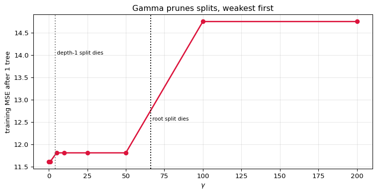
Raising $\gamma$ therefore prunes the tree from the bottom up: weak splits vanish first, and at a high enough $\gamma$ the tree collapses to a single leaf that predicts the mean.
gamma   splits kept   leaves   train MSE
--------------------------------------------
       0             2        3     11.6105
       1             2        3     11.6105
       5             1        2     11.8060
      10             1        2     11.8060
      25             1        2     11.8060
      50             1        2     11.8060
     100             0        1     14.7514
     200             0        1     14.7514
--------------------------------------------

the root split's gain is 66.292 (xgboost scale), so it survives
every gamma below that and disappears once gamma exceeds it.
the depth-1 split's gain is 4.302, so it is pruned much earlier.
9. Learning Rate and the Number of Trees
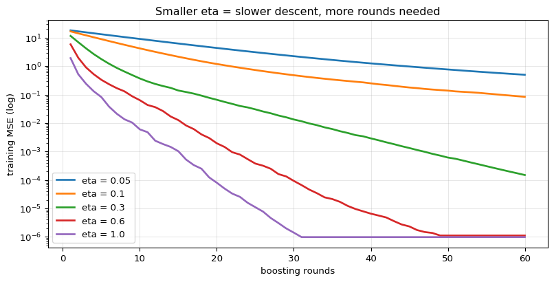
$\eta$ and num_boost_round trade against each other: a smaller learning rate needs
more trees to reach the same fit, but usually generalises better because no single tree
dominates.
eta        r=1        r=5       r=10       r=25       r=50
------------------------------------------------------------
  0.05    18.1988    13.2988     9.0930     3.1069     0.7685
   0.1    16.7493     8.9155     4.2276     0.7334     0.1388
   0.3    11.6105     1.7745     0.3704     0.0304     0.0006
   0.6     5.8795     0.3326     0.0637     0.0004     0.0000
   1.0     1.9291     0.0819     0.0060     0.0000     0.0000
------------------------------------------------------------

These are TRAINING curves on 12 rows, so they all march to zero - that is
overfitting, not success. On real data the validation curve turns back up,
and the smaller eta usually turns up later and lower.
10. Summary
| Stage | Formula | Value in round 1 |
|---|---|---|
| Gradient | $g_i = \hat y_i - y_i$ | $\sum g = -38.7$ |
| Hessian | $h_i = 1$ | $\sum h = 12$ |
| Leaf weight | $w^{*} = -\dfrac{G}{H+\lambda}$ | root would be $+2.977$ |
| Similarity | $\dfrac{G^2}{H+\lambda}$ | $115.16$ |
| Split gain | $\tfrac12\big[S_L + S_R - S_P\big] - \gamma$ | $33.15$ (xgb prints $66.29$) |
| Shrinkage | output $= \eta\, w^{*}$ | $\eta = 0.3$ |
The one idea: approximate the loss by a quadratic, and a quadratic has a closed-form minimum. That is why XGBoost never needs to guess a leaf value or score a split heuristically — both drop out of the same two sums, $G$ and $H$.
Why second order matters: for squared error $h_i = 1$ and the Hessian looks like bookkeeping. For logistic loss $h_i = p_i(1-p_i)$, which is small for confident predictions — so the Hessian automatically down-weights rows the model has already settled, something first-order gradient boosting cannot do.
What is deliberately left out: the sparsity-aware default direction for missing
values, min_child_weight (a floor on $H$ per leaf), column and row subsampling,
approximate/histogram split finding, and multi-class objectives.
What comes next: LightGBM and CatBoost keep this exact gain formula and change how the tree is searched — histograms and leaf-wise growth in one, ordered statistics and oblivious trees in the other.